Adaptive Sampling technical guide (ADS_S1016_v1_revQ_11Nov2026)


Protocol
V ADS_S1016_v1_revQ_11Nov2026
FOR RESEARCH USE ONLY.
Contents
Adaptive Sampling
Introduction
- 2. How Adaptive Sampling works
- 3. Low-pass whole genome and methylation sequencing
- 4. Defining concepts and vocabulary
- 5. Files and equipment required
Adaptive Sampling protocols
- 6. Choosing an Adaptive Sampling protocol
- 7. Protocol selection
- 8. Ultra-rapid singleplex
- 9. Singleplex
- 10. Multiplex
Digital Panel Designer
- 11. Designing a panel with the Digital Panel Designer
- 12. Choosing the reference assembly
- 13. Adding your targets
- 14. Reviewing the target table
- 15. Setting the buffer
- 16. Summary and export
- 17. Known limitations
Library preparation
MinKNOW
Monitoring and troubleshooting
- 23. Rejection peak length
- 24. Slow decisions
- 25. Bimodal rejection peak
- 26. Failed reads
- 27. Target confirmation
- 28. Comparing two runs
Reference
- 29. How Adaptive Sampling decides
- 30. The decision process
- 31. Buffers, targets and footprint
- 32. Library length
- 33. Strand directionality
- 34. Depletion mode
- 35. Device limits
Appendix
- 36. Appendix A — designing a panel without the Digital Panel Designer
- 37. Appendix B — output files and field definitions
FAQs
1. Overview
Adaptive Sampling is an on-device real-time targeted sequencing approach from Oxford Nanopore. Rather than relying on probe or amplicon-based target enrichment panels, Adaptive Sampling uses BED-file-based digital panels to define the genomic regions you want to enrich during sequencing. As sequencing begins, native DNA molecules enter the nanopores and are assessed in real-time against the digital panel. Molecules containing regions of interest continue to be sequenced, while those not containing regions of interest are ejected from the nanopores. This increases coverage across targets, generates low-pass whole-genome data from off-target reads, and preserves methylation information, giving you targeted and genome-wide genetic and epigenetic insights from the same run.
This guide takes you through designing a panel, preparing your library, setting up the sequencing run, and interpreting the result. You can either begin with one of our ready-to-use digital panels or design a custom panel with our Digital Panel Designer. Add your targets of interest (gene name, coordinates, BED file) or modify one of our ready-to-use panels using the Digital Panel Designer. This tool will then output all necessary files for sequencing and some useful files for downstream coverage and variant analysis.
Sections 2 to 28 cover the experiment itself, in the order in which you will carry it out. Sections 29 to 35 are reference material describing the mechanisms behind the decisions made during a run and is intended for occasions when a run does not behave as you expect. Appendix A describes the manual design route which remains available for cases the Digital Panel Designer tool does not cover. Sections 39 to 44 cover frequently asked questions regarding the Digital Panel Designer.
2. How Adaptive Sampling works
As each DNA strand enters a pore, the first 450 bases or so are basecalled and aligned in real-time. At a sequencing speed of 450 bases per second, this initial assessment takes approximately one second. If the sequence aligns to a region of interest defined in the provided BED file, sequencing continues for the strand. If the sequence does not align to a region of interest, the voltage across the pore is reversed to eject the strand, freeing the pore to sequence another DNA molecule.
Over the course of the run, this process directs more of the flow cell output towards the regions of interest, increasing sequencing depth and coverage. The approximate 450 bp reads generated from rejected strands are also aligned, providing low-pass whole-genome coverage.
Adaptive Sampling operates in two modes:
Enrichment: The BED file defines the regions to sequence. Strands that align within these regions are accepted and sequencing continues. Strands that align outside these regions or do not align to the reference are rejected.
Depletion: The BED file defines the regions to exclude from sequencing. Strands that align within these regions are rejected. All other strands, including those that align outside the defined regions or do not align to the reference are accepted and sequencing continues.
Enrichment is the mode we have optimised and validated, and this guide assumes it. Depletion is supported, but it has not been validated to the same extent. Depletion is intended for enriching sequences you are unable to name in advance, by subtracting the genomes you already know to be present. Rare or unknown sequences then receive the available pore time. Depletion mode is described in section 34.
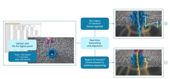
Figure 1: Overview of an Adaptive Sampling experiment. The BED file defining your digital panel is uploaded to MinKNOW. As each strand enters a pore, the first ~450 bases, about one second of sequencing, are basecalled and aligned in real-time. A strand outside the regions of interest is rejected and the pore is freed for the next strand; a strand inside the regions is allowed to continue sequencing.
3. Low-pass whole genome and methylation sequencing
The strands which are rejected are still basecalled and still written out, so an enrichment run returns a low-pass view of the whole genome alongside the enriched targets, from the same flow cell and at no additional cost in sample or preparation. In the Hereditary Cancer Panel, the targeted genes reached 36 to 65-fold coverage while the rest of the genome was covered 3 to 5-fold. That is enough depth to call copy number changes and large structural rearrangements genome-wide.
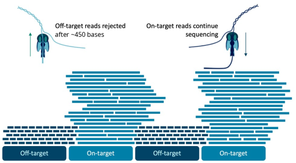
Figure 2: Targeted answers alongside genome-wide data. Strands outside the targets are rejected after about 450 bases, while strands inside them continue sequencing. Targets therefore reach high coverage and the rejected reads give a low-pass view of the whole genome and its methylation.
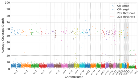
Figure 3: Average coverage depth across each chromosome in an enrichment run. Targets are covered at around 50-fold, while the rest of the genome is covered at low depth by the rejected strands, which are still basecalled. The dashed lines mark 20 and 30-fold coverage depths.
The library is prepared from native DNA and is never amplified. Base modifications are preserved in the signal and are called in the same run. A single Adaptive Sampling experiment therefore returns three layers of data: high coverage across the regions you asked for, a low-pass whole genome, and methylation across both. You can choose Adaptive Sampling over a physical panel even where a physical panel exists for your application. Plan the analysis for all three layers before the run, rather than after it.
4. Defining concepts and vocabulary
Digital panel: A digital panel is the set of target regions you define in a BED file, and it is the term used throughout the product literature. The contrast is with a physical panel of primers or probes, which is fixed once it has been ordered, whereas a digital panel can be rebuilt in minutes with targets added or removed. Where this guide refers to the BED file, the BED file is the digital panel.
ROI (region of interest): The ROI is the region you are interested in, excluding any buffer you add around it.
Buffer region: Buffer regions are added to the 5′ end of every ROI on both the plus and the minus strand, so the enrichment BED file has two rows for each ROI. The decision to accept or reject a strand is made on the first 450 bases or so only. A strand which begins upstream of your ROI would go on to sequence through it but will be rejected unless the buffer covers the position at which that strand began. Adding buffer is therefore what prevents you from losing those reads, and it is also what evens out the coverage obtained at the edges of your ROIs. Buffer is not added to the 3′ end, since a strand which begins past the ROI is reading away from it. Section 33 describes the mechanism.
Target: The target is the ROI plus its buffer region, and it is the total amount of sequence against which Adaptive Sampling makes its decision. The size of the target, rather than the size of the ROI, is what determines the degree of enrichment you will obtain.
Footprint: The footprint of a panel is the size of its target expressed as a percentage of the genome. This is the single most useful number for predicting how a panel will perform. The smaller the footprint, the more sample the pores can sample through to find it. Note that the footprint of a panel is not the same as the size of its ROIs. For panels containing a large number of small targets, buffer usually accounts for most of the footprint. The Digital Panel Designer reports the footprint as the proportion of the genome covered on either strand. As each strand has buffer at the 5′ end only, the amount selected on any one strand is somewhat smaller than this figure.
When calculating the percentage of a sample targeted by Adaptive Sampling, you need to take the prevalence of the targeted regions within the sample into account. Consider an E. coli genome spiked into a human sample, where you are targeting 50% of the E. coli genome. The E. coli genome represents only 10% of the total DNA present. Therefore, you are targeting 5% of the sample, not 50%.
5. Files and equipment required
Adaptive Sampling requires the following inputs:
A genomic reference in FASTA format which represents the complete sample, and not only the regions you intend to target. A reference which omits sequence present in the sample will cause some strands not to align at all and will also increase the likelihood of false positive alignments. If your sample contains more than one organism, download a reference for each of them and concatenate the files. Before you do so, check the contig names for duplication, as a sequence named 'chr1' in two of the constituent references will cause misalignment.
The coordinates of your regions of interest in a BED file, including buffer where applicable. The contig names used in the BED file must match those used in the reference exactly.
A device with a compute that is capable of basecalling, aligning and deciding on every strand, while the run proceeds. The PromethION 2 Integrated and PromethION 24 are the recommended devices for Adaptive Sampling.
The Digital Panel Designer produces the interval files from a list of gene names as described in the section on the Digital Panel Designer. The reference itself is not produced by this tool, so download it separately and keep it alongside the panel for the life of the project. Appendix A (section 36) describes the manual route for cases the tool does not cover.
The contig name in the reference is the text in the FASTA header up to the first space. It must appear in the first column of the BED file exactly as it is written. An example is shown here:
>chr1 CP068277.2 Homo sapiens isolate CHM13 chromosome 1
CACCCTAAACCCTAACCCTAACCCTAACCCTAACCCTAACCCTAACCCTAA...

chr1    45311243    45358470    MUTYH_region
chr1    114686464   114734788   NRAS_region
A reference downloaded from Ensembl names the same chromosome 1 rather than chr1, and a BED file written against a UCSC reference will not match it. Where the names differ, rename the BED file. Do not rename the reference. Rename every contig you intend to target.
For human panels, we recommend the GRCh38 no-alt analysis set from NCBI (GCA_000001405.15_GRCh38_no_alt_analysis_set). Its contigs are named in the form chr1, which is the form the Digital Panel Designer writes into its BED files, and the files from the tool can therefore be loaded alongside it without renaming. The Ensembl GRCh38 reference names the same contig 1 and will not match them, even though the tool uses Ensembl to locate genes.
For the Hereditary Cancer Panel, we recommend the Genome in a Bottle (GIAB) v3 GRCh38 reference, which was used to establish the performance of the panel. GIAB v3 is the no-alt analysis set with falsely duplicated regions masked and decoy sequences added. It keeps the same contig names and coordinates, so BED files designed on GRCh38 in the Digital Panel Designer work with either reference.
In GRCh38, some genes have a false second copy or are missing a real copy. Reads from these genes cannot be placed reliably, which can reduce enrichment and cause false variant calls. GIAB v3 corrects this for CBS, U2AF1, CRYAA and KCNE1, whose false copies on chromosome 21 are masked so that reads align to the true gene, and for MAP2K3, KMT2C and KCNJ18, where reads from copies missing from GRCh38 align to decoy sequences instead of the target gene. If your panel includes any of these genes, use GIAB v3.
Avoid references that include alt contigs, such as full GRCh38 with HLA alternates. Reads that align to an alt contig fall outside the BED file and are rejected. Some GRCh37 (hg19) references contain haplotype contigs in the MHC region, and the same caution applies to panels with targets there. Use the same reference FASTA for downstream analysis as you load into MinKNOW.
Reference FASTA files for panels:
| Panel | Build | Reference FASTA file | Source |
|---|---|---|---|
| All other panels | GRCh38 | GCA_ 000001405. 15_ GRCh38_ no_ alt_ analysis_ set. fna. gz | NCBI |
| Hereditary Cancer and Pan-Cancer Panels | GRCh38 | GRCh38_ GIABv3_ no_ alt_ analysis_ set_ maskedGRC_ decoys_ MAP2K3_ KMT2C_ KCNJ18. fasta. gz | Genome in a Bottle |
| Custom panels | GRCh37 | hg19. p13. plusMT. no_ alt_ analysis_ set. fa. gz | UCSC |
We do not advise pre-indexing your reference files before uploading them to MinKNOW. In the latest version of MinKNOW, the software indexes the reference automatically at the beginning of the run. It uses parameters that we keep under review. These parameters optimise the speed and accuracy of Adaptive Sampling alignment. A reference which you have indexed yourself will most likely not have been indexed with the same parameters, and this can affect the Adaptive Sampling decision, leading to both false positives and false negatives.
6. Choosing an Adaptive Sampling protocol
Three protocols are supported for Adaptive Sampling. They differ in the number of samples which share a flow cell and in how quickly a result is required, and that choice in turn constrains the size of the panel you can design, the way you prepare your library, and the sequencing device you run on. In all three protocols, the flow cell is run once and should not be washed and reused, since there is too little sequencing capacity left for a second run.
| Ultra-rapid singleplex | Singleplex | Multiplex | |
|---|---|---|---|
| Intended use | Somatic work where time to result is the main constraint | Somatic work on one sample per flow cell, with sample tracking | Germline work, in batches of three samples |
| Samples per flow cell | 1 | 1 | 3 |
| Library preparation kit | Ligation Sequencing Kit (SQK-LSK114) | Native Barcoding Kit (SQK-NBD114.24) | Native Barcoding Kit (SQK-NBD114.24) |
| Barcoding | None | One barcode, used for sample tracking | Three barcodes, pooled before adapter ligation |
| Flow cell | PromethION Flow Cell (FLO-PRO114M) | PromethION Flow Cell (FLO-PRO114M) | PromethION Flow Cell (FLO-PRO114M) |
| Devices supported | PromethION 24 PromethION 2 Integrated | PromethION 24 PromethION 2 Integrated | PromethION 24 PromethION 2 Integrated |
| Time to result | Methylation classification after 30 minutes of sequencing, or once ~0.75 Gb of pass data has been generated. | 72 hours | 72 hours |
| Library preparation time | ~65 minutes | ~2 hours 20 minutes | ~3 hours 20 minutes |
| DNA input* | 1 µg of sheared gDNA | 500 ng to 1 µg of sheared gDNA | 1 µg of sheared gDNA per sample |
| Fragmentation | Covaris g-TUBE fragment length ~7.5–8 kb | Covaris g-TUBE fragment length ~7.5–8 kb | Covaris g-TUBE fragment length ~7.5–8 kb |
| Typical library N50 | 8–10 kb | 8–10 kb | 8–10 kb |
| Recommended panel footprint | 0.1–5% of the genome | 0.1–5% of the genome | 0.1–5% of the genome |
| Recommended buffer | 20 kb at the 5′ end, plus and minus strands | 20 kb at the 5′ end, plus and minus strands | 20 kb at the 5′ end, plus and minus strands |
| Expected on-target coverage | >75x for a 5,000 pore PromethION Flow Cell | >75x for a 5,000 pore PromethION Flow Cell | 90% of target bases >20x (30x mean coverage per sample) |
| Basecall on-target reads only (BOTO) | Off | Off | Optional On: rejected reads are not basecalled, which frees the compute to run more flow cells at the same time. Off (the protocol default): fewer flow cells can be run at the same time, but the off-target reads give low-pass whole-genome and methylation data. |
*Refer to the specific protocols for more information.
7. Protocol selection
The protocol follows from the application and the number of samples. Where time to result is the main constraint, for example, tumour classification within hours, use Ultra-rapid singleplex. For somatic work on one sample at a time, where the sample needs to be tracked through the run, use Singleplex. For germline samples which can be batched in groups of three, use Multiplex.
Once the protocol is chosen, check that the footprint of your panel, as reported by the Digital Panel Designer, lies between 0.1 and 5% of the genome, and that you can obtain high-molecular-weight DNA which can be sheared to the fragment length the protocol specifies.
8. Ultra-rapid singleplex
Ultra-rapid singleplex uses the Ligation Sequencing Kit without barcoding and runs one sample on each PromethION Flow Cell. It gives the shortest time to result of the three protocols and is intended for somatic work in which a result is needed within hours. Methylation-based classification can be performed after 30 minutes of sequencing, or once ~0.75 Gb of pass data has been generated. Sequencing can then continue for up to 72 hours to build depth across the targets for variant calling.
9. Singleplex
Singleplex uses the Native Barcoding Kit and runs one sample on each flow cell, with the barcode used to track the sample rather than to pool samples. It is used with the Pan-Cancer Panel on fresh or frozen tumour tissue however, FFPE samples are not supported. With the Pan-Cancer Panel, the targeted protocol gives a median coverage above 75-fold across the targets, and SNVs, indels, copy number changes, structural variants and methylation are called from the same library.
10. Multiplex
Multiplex uses the Native Barcoding Kit to pool three barcoded samples on one PromethION Flow Cell. It is the protocol for the Hereditary Cancer and Pharmacogenomics Panels and for custom germline panels. DNA is extracted from whole blood and sheared with a Covaris g-TUBE to 7.5–8.5 kb, and each sample is ligated to its own barcode before the three are pooled for adapter ligation. On the Hereditary Cancer Panel, the protocol gives more than 30-fold mean coverage on every target gene for each sample, with 3 to 5-fold coverage across the rest of the genome.
The three samples share the pores of one flow cell, so the footprint of the panel is interpreted as it would be for a single sample, and the output of the flow cell is divided between the three. Uneven representation of the barcodes lowers the coverage of the weakest sample. Therefore, we recommend quantifying each library accurately before pooling.
Custom panels differ in size, gene content and sequence context, so the coverage your panel reaches may differ from that of the ready-to-use panels. We recommend running a pilot with your panel and confirming the coverage you need before processing large numbers of samples.
Load 250 to 300 ng of the pooled library, since loading less than 250 ng lowers pore occupancy. The flow cell is run for 72 hours with 5mC and 5hmC calling switched on, and it should not be washed and reused afterwards, since there is too little sequencing capacity left for a second run.
11. Designing a panel with the Digital Panel Designer
The Digital Panel Designer converts a list of genes, coordinates or an existing BED file into the files a sequencing run requires, and it is the route we recommend for every panel. It replaces the procedure described in Appendix A, so you no longer need the UCSC Table Browser, a local conda environment, samtools, bedtools, or the buffer arithmetic described in section 31. It also reports the footprint of the panel as you build it, which is the number that predicts how the panel will perform, and it writes the files in the form MinKNOW expects.
The tool takes you through three steps, shown across the top of the window: Target Input, Buffer Configuration, and Summary and Export. You can move between them with Back and Next at any point, and the summary on the right of the window updates as you work, so the footprint of the panel is visible before you commit a flow cell to it. Sections 12 to 14 below cover the first step, in which you choose the reference assembly, add your targets, and review what the tool made of them. Sections 15 and 16 cover the second and third steps respectively.
The manual route in Appendix A remains available and is the one to use if your organism has no gene model in either Ensembl or NCBI, or if you are targeting classes of annotation which the tool does not resolve, such as repeats, regulatory features or structural variant catalogues, or if the machine on which you design your panel has no network access.
12. Choosing the reference assembly
Select your assembly before you add any targets. A gene which has been located is an answer about one build only: the position chr17:83,000,000 is a real position in GRCh38 but lies beyond the end of the contig in GRCh37. Changing the assembly therefore clears the panel, and the tool tells you so, since targets placed against one build cannot be carried over to another. Choose the assembly first, and if you change it, add your targets again.
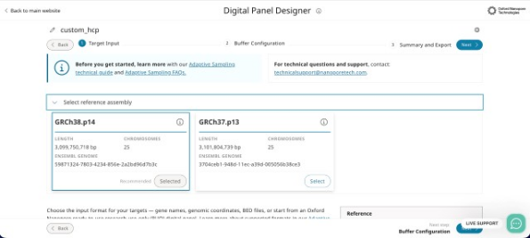
Figure 4: Selecting the reference assembly at the top of the Target Input step. Each card gives the length of the assembly, the number of chromosomes and the Ensembl genome identifier, and the assembly marked 'Recommended' is selected by default.
The assembly you select here must correspond to the reference FASTA you load into MinKNOW. Mismatched builds are the most common cause of a panel which targets the wrong sequence while running without any apparent error. The patch level is given on each card, GRCh38.p14 and GRCh37.p13 at the time of writing, and it is worth recording alongside your run.
13. Adding your targets
There are four ways of adding targets on the tabs beneath the assembly cards, and you can use more than one of them within a single panel.
Preset Panel: Select one of the Oxford Nanopore ready-to-use research-use-only digital panels from the dropdown and load it. The description and the number of targets are shown before you load. Targets from a ready-to-use panel can be removed but not edited, and you can add your own targets alongside them. A preset is a starting point rather than a fixed list. This is the quickest route to a working panel, and the one to use where a ready-to-use panel covers your application. At launch, the Hereditary Cancer, Pharmacogenomics and Pan-Cancer Panels are available, and the Pan-Haematological Cancer Panel will follow.
Each panel is offered in two forms:Panel (Targets + Buffer) starts from the panel as supplied, with its buffer fixed at the panel’s own width. A panel loaded in this form must be customised by adding or removing at least one target, before it can be exported:
- 10 kb for Hereditary Cancer
- 20 kb for Pharmacogenomics
- 20 kb for Pan-Cancer
Targets Only carries the targets alone. The buffer is set in the Buffer Configuration step at the default of 20 kb unless you change it.
Load Targets Only if you want to set the buffer to suit your library, and Targets + Buffer if you want to adjust the panel while keeping its supplied buffer. To use a ready-to-use panel exactly as supplied, without changes, download its enrichment BED file, with checksums, from the link given in the tool, rather than exporting it from the Digital Panel Designer.
Gene Input: Type or paste a list of gene names. Each symbol is looked up first in Ensembl. A symbol filed under another name is then resolved through HGNC, and then through the Ensembl gene identifier, and NCBI Gene is consulted last. A gene target covers the whole gene, from the lowest start to the highest end across all its transcripts. Most users can leave the gene target as it is. For advanced users, the optional Pick transcripts control narrows the target to selected transcripts, for example the MANE Select or protein-coding transcripts and Choose gene model selects between models where Ensembl holds more than one for the symbol. Each row records which service placed it. RefSeq and Ensembl coordinates can disagree by as much as a few kilobases for genes which both services know, and that difference is worth reviewing before you export.
Coordinates: Enter coordinates in the form chr17:43044295-43125364, one region per line. Use the These coordinates are dropdown to declare whether they are 0-based, half-open (BED), which is the default, or 1-based, inclusive, the convention used by IGV, the UCSC Genome Browser and Ensembl. The two readings differ by one base at the 5′ end and nothing downstream of this point can detect the error. A one-base shift is always within bounds and always well formed.
BED File: Upload an existing panel, whether from a previous run, from a collaborator, or from the Adaptive Sampling Catalogue on Nanopore community and edit it in the table.
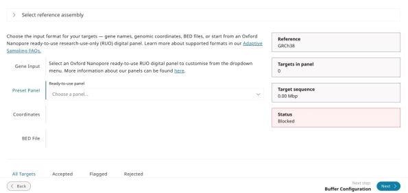
Figure 5: The Target Input step with 'Preset Panel' selected. Choose a ready-to-use panel from the dropdown to load it as the starting point for your panel, which you can then edit.
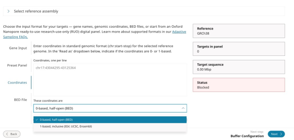
Figure 6: The Target Input step with 'Coordinates' selected. Coordinates are entered one per line, and the 'These coordinates are' dropdown sets whether they are read as 0-based, half-open (BED), the default, or 1-based, inclusive, as used by IGV, UCSC and Ensembl. The summary on the right reports the reference, the number of targets in the panel, the length of the target sequence, and a status which reads as 'Blocked' until the panel contains targets that can be exported.
The ready-to-use panels available at the time of writing are listed below. Any of them can be loaded in the Digital Panel Designer as a starting point for a custom panel. Unedited ready-to-use panels cannot be exported from the tool. To use a panel exactly as supplied, download its BED files from the Adaptive Sampling webpage.
| Digital panel | Research application | Targets | Sequencing protocol | Analysis | Status |
|---|---|---|---|---|---|
| Hereditary Cancer | Cancer predisposition | 258 genes (259 targets) | Multiplex | wf-hereditary-cancer | Available at launch |
| Pharmacogenomics | Drug response | 375 genes | Multiplex | wf-pgx | Available at launch |
| Pan-Cancer | Tumour profiling | 723 genes | Singleplex or Ultra-rapid singleplex | Command line, refer to the bioinformatics guide | Available at launch |
| Pan-Haematological Cancer | Haematological malignancies | 144 genes | Singleplex | Command line, refer to the bioinformatics guide | Coming in Dec 2026 |
Target counts are those published in the Getting started guide, and panel revisions change these counts over time. Read the count the tool reports for the panel you have loaded. The table above does not reflect these changes.
Custom panels, and ready-to-use panels which you have edited, are analysed with the wf-human-variation workflow for germline applications or by following the Somatic analysis bioinformatics guide.
14. Reviewing the target table
Every target the tool has placed appears in the table below the input tabs, and the tabs above it divide the rows into those which were accepted, those which have been flagged for a second look, and those which were rejected. Each row gives the status, the source which placed it, the name, the locus with its length in base pairs, and any notes. Rows can be searched by name, alias or coordinate, and can be removed individually.
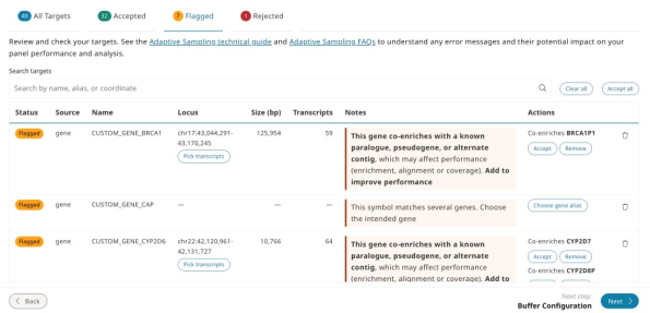
Figure 7: The Flagged tab of the target table. Each flagged row gives the reason in the Notes column and the Actions available: accepting or removing a co-enriched paralogue, pseudogene or alternate contig, choosing the intended gene where a symbol is ambiguous, or picking transcripts.
Two things that are worth reviewing before you move on:
Flagged rows: A flag means the row needs a decision from you before the panel can be exported. Two conditions are grouped under one review error, and export is blocked until you accept or remove each row concerned. The first is co-enrichment, where a target has paralogues, pseudogenes or alternate contigs similar enough that reads from them will also be accepted. The tool names the co-enriched gene, and where the partner can be added, it offers Add to improve performance. The second is a duplicate interval, where the same region has been added under two names. Co-enrichment is a property of the genome rather than of your panel, but it affects how the coverage at those loci should be read, and it is better known before a run than after one. A flag is also raised where a gene symbol matches more than one gene, in which case Choose gene alias lists each candidate with its location, size and source, and you can pick the one you intended.
Rejected rows: A rejection means the tool could not place the row and the reason is given in the table rather than the row being discarded silently. A name which no service recognises, a coordinate beyond the end of a contig and a malformed BED line all appear here. Rejected rows are not written to the export, so the count on the Rejected tab is the number of targets you asked for but will not receive and it is worth resolving before you proceed.
The messages given for coordinates, BED lines and gene names that cannot be placed are listed below:
| Message | What to do |
|---|---|
| not BED: needs chromosome, start and end as the first three columns | Check the file is tab-separated and starts with chromosome, start and end. |
| not written as chr1:1000-2000, chr1 1000 2000 or chr1:1000 | Re-enter the coordinate in one of these three forms. |
| position 0 does not exist in 1-based coordinates | Set the dropdown to 0-based or correct the start position. |
| chromosome not in the reference genome | Check the chromosome name against the selected assembly, for example, chr1 rather than 1. |
| past the end of {chrom}, which is {length} bp | Check the coordinate belongs to the selected assembly. |
| start is not before end | Swap the start and end positions. |
| not a valid gene symbol | Use the HGNC approved symbol for the gene. |
15. Setting the buffer
The buffer control adds flanking sequence to the 5′ end of every ROI on both the plus and the minus strands, as described in section 33. The default is 20 kb and it can be adjusted between 10 kb and 30 kb in steps of 1 kb. The footprint of the panel is recalculated as you move the control.
Two lines beneath the control report what the buffer has done. The first gives the number of design rows, with the number of flanks shortened where a buffer meets a neighbouring target and the number collapsed at the end of a contig. The second gives the footprint twice: summed over all targets, and as a unique sequence, which counts any region covered by more than one row once. The percentage of the genome is calculated from the unique figure.
Set the buffer from the read length distribution of your library. As a guideline, a value between the N25 and the N10 of that distribution is a good starting point. Longer libraries require more buffer. The more targets a panel contains, the more footprint a given buffer will cost you. Buffer is added to each region individually. Section 31 explains this trade-off in full, including the case where shearing the library shorter is a better solution than reducing the buffer.
Rows belonging to different targets are not merged. Where two targets lie close together, a buffer is shortened so that it stops at the start of the neighbouring target. Where two targets overlap, or one contains the other, both buffers are added in full, so buffers belonging to different targets may overlap. The reported footprint counts any sequence covered by more than one row once. Section 31 describes these cases in full.
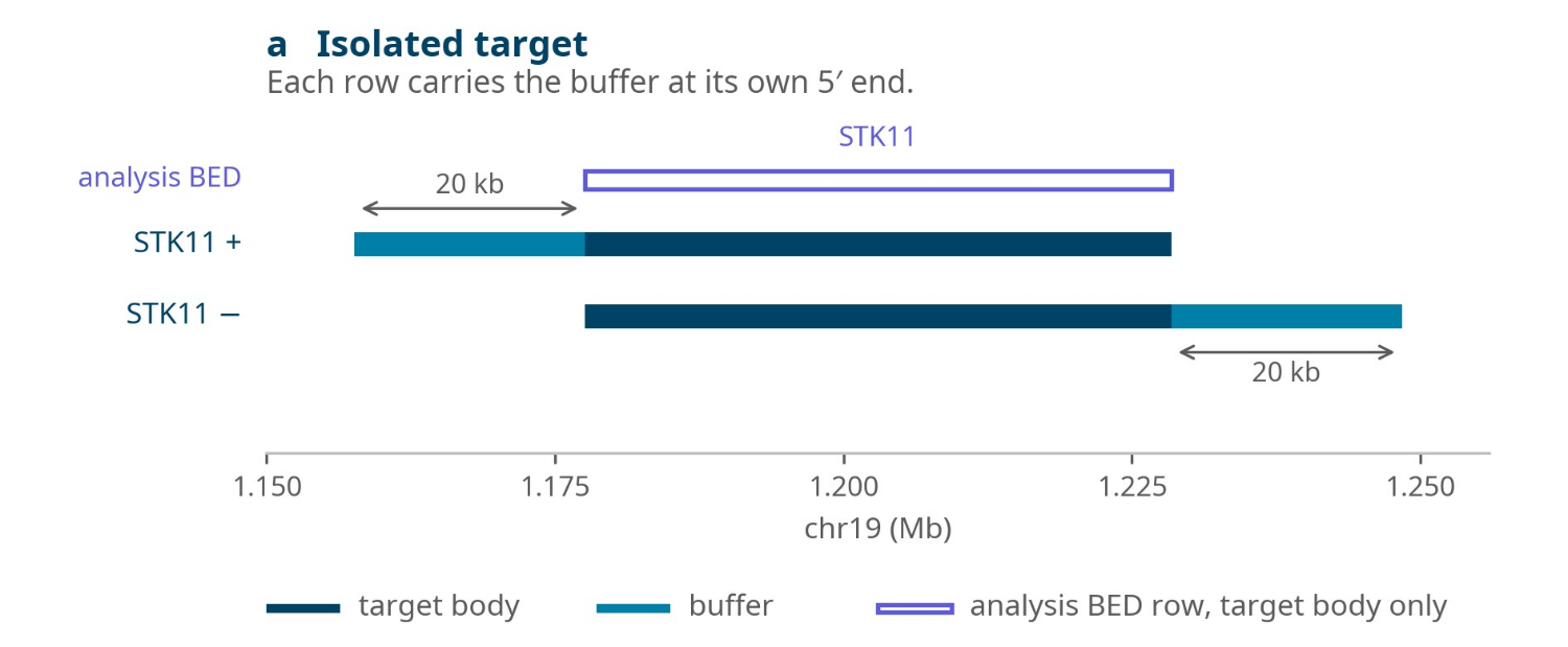
Figure 8: Buffer applied to an isolated target, STK11, at the default of 20 kb. The plus strand row of the enrichment BED file carries the buffer before the target. The minus strand row carries it after the target, and the analysis BED file carries the target alone.
Buffer is clamped at the ends of each contig, so a target lying near a telomere receives as much buffer as the contig can provide.
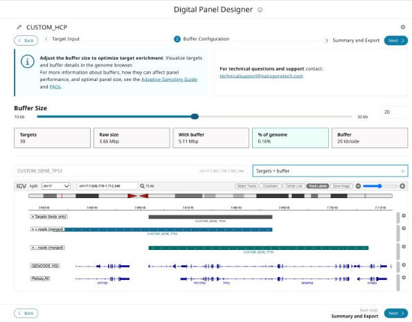
Figure 9: The Buffer Configuration step for TP53 at the default of 20 kb. The tiles report the number of targets, their length with and without buffer, and the footprint. The genome browser shows the target body, the plus strand row extending 20 kb upstream of it, and the minus strand row extending 20 kb downstream.
16. Summary and export
The summary step restates what the panel contains and what it will cost you. The footprint is given both as a length and as a percentage of the genome, and it is the figure which predicts how the panel will perform. A panel below approximately 5% is comfortable. Above this figure, enrichment begins to fall away. Between 5% and 10%, the tool shows a large-panel warning, but the panel can still be exported. The pores spend an increasing proportion of the run sequencing accepted off-target flanking sequence. If your panel is above 5%, you can reduce the buffer, remove targets, or shear the library shorter.
Note that panels with a footprint below 0.1% of the genome, or above 10%, are prevented from exporting. The lower limit is intended to catch panels which are too small to enrich usefully and the upper limit to catch panels large enough that Adaptive Sampling will not improve on a standard sequencing run. Both are design-time safeguards. The device does not impose these limits.
The export produces the following files:
| File | Content | Where it is used |
|---|---|---|
| *_enrichment.bed | ROI plus buffer at the 5′ end, one row each for the plus and minus strand | MinKNOW, the Adaptive Sampling BED field |
| *_analysis.bed | ROI only, without buffer | Secondary analysis |
| *_exons.bed | One row per exon of the MANE Select transcript, or the Ensembl canonical transcript where there is none | Downstream coverage analysis |
| summary.html | Panel statistics and design checks | Your run record |
*_enrichment.bed
This is the file MinKNOW needs for Adaptive Sampling, as described in section 21. It contains two rows for each ROI, one for the plus strand and one for the minus strand, each with buffer at the 5′ end.
*_analysis.bed
This carries the same regions without their buffer, and it is for secondary analysis after the run: calculating coverage over your ROIs, restricting variant calling to them, and any other downstream step which should see your targets rather than your targets plus their flanking sequence. It is not a sequencing input and it is not loaded into MinKNOW.
*_exons.bed
This gives one row for each exon of the MANE Select transcript of each gene, or of the Ensembl canonical transcript where a gene has no MANE Select transcript for coverage analysis. An exon which cannot be placed is reported in the file rather than left out.
summary.html
This is a self-contained report of the panel. It gives the panel specification, the results of the design checks, the list of exported files and the full target table, with an interactive genome browser view of the targets and their buffers. It opens in any web browser without a network connection. None of the BED files record the reference assembly or the buffer size, so keep the summary.html with them as a record of how the panel was designed. This is the information you are likely to want when one run is compared with another some months later.
The files are named by date and panel name, in the form:
YYYY-MM-DD_panel-name_enrichment.bed
Two errors in the use of these files which are seen most often:
If *_analysis.bed is loaded into MinKNOW in place of *_enrichment.bed, the run has no buffer, strands which begin upstream of each ROI are ejected, and enrichment falls.
If coverage is calculated over *_enrichment.bed in place of *_analysis.bed, the result includes the buffer and no longer describes your ROIs.
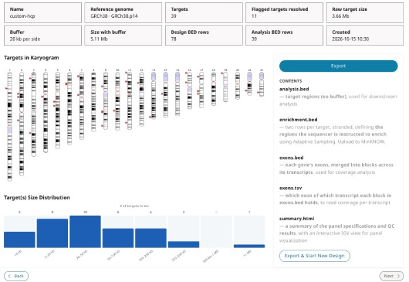
Figure 10: The Summary and Export step. The tiles restate the design, including the number of rows in the enrichment and analysis BED files, the karyogram and size distribution show where the targets lie, and the panel on the right lists the files written by Export.
17. Known limitations
The following limitations apply to the release of the Digital Panel Designer described in this guide:
Targets which fall in gaps in the assembly, or which have no exon model, cannot be given exon intervals. These are reported in *_exons.bed rather than left out silently. VKORC1P2 is one example. We recommend checking *_exons.bed for unplaced exons before you calculate coverage.
Panels with a footprint below 0.1% of the genome cannot be exported. A panel of BRCA1, BRCA2 and TP53 falls below this limit at 0.012%. For panels of this size, use the manual route in Appendix A.
18. Preparing the library
Although Adaptive Sampling does not require any particular sample preparation, there are two properties of the library which determine how much data you obtain from the run: pore occupancy and library fragmentation.
19. Pore occupancy
The Adaptive Sampling methodology is based on rejecting unwanted strands. This frees the pore for a new strand and reduces the proportion of the run for which each pore is occupied. Maintaining high pore occupancy is therefore one of the most important considerations in an Adaptive Sampling experiment.
We recommend loading a higher amount of sample than you would use for a standard sequencing run. Calculate the amount to load from the point of view of molarity rather than mass. The number of DNA ends available for capture governs the rate at which pores are refilled. The ideal molarity when using the latest V14 chemistry is 50 to 65 fmol per load.
Qubit is the recommended method for evaluating the concentration of your library. The result should then be converted into a molarity using the average fragment length of the library. You can evaluate fragment length using the Agilent Femto Pulse System for fragments above 10 kb, or the Agilent Bioanalyzer for fragments below 10 kb. Using the average molecular weight of a base pair (660 g/mol), the molarity is straightforward to calculate. For a library with a read length distribution centred on 6.5 kb (Figure 11), 50 fmol corresponds to approximately 200 ng:
Total mass of a mole of 6.5 kb fragments: 6,500 bp x 660 g/mol = 4,290,000 g
Multiply by the number of femtomoles: 4,290,000 x 50 x 10-15 = 2.145 x 10⁻⁷g
Convert grams to nanograms: 2.145 x 10-7 x 109 = 214.5 ng
To facilitate these calculations, you can use a biomath calculator such as the following from Promega.

Figure 11: Read length distribution of a library with an N50 of 6.5 kb.
This is a rough approximation based only on the N50 of the library. The true molarity is more intricate to calculate, since you need to take the range of the read length distribution into account. Nevertheless, it is a good approximation for understanding the amount of DNA you will need. These values also assume optimal ligation efficiency. However, if there is any reason to suspect that a library is not ligating efficiently, we advise adding a further amount of sample. Note that a higher DNA input has not been shown to affect the run adversely.
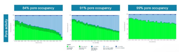
Figure 12: Pore activity in MinKNOW for three runs at 84%, 91% and 99% pore occupancy. The higher the occupancy, the larger the proportion of the array that is sequencing (green) rather than waiting for a strand.
20. Library fragmentation
Shorter libraries are generally preferable for Adaptive Sampling for three reasons.
Pore blocking: Adaptive Sampling runs are more likely to block pores than standard runs. The rate of strand rejection is high. Longer fragments block pores more severely. Figure 13 (below) shows the number of pores available for sequencing over the course of two runs, using libraries of 6 kb and 20 kb. Attrition of channels occurs at a noticeably faster rate in the library with the longer fragments.
Molarity: A shorter library provides a higher molarity equating to more available DNA ends for the same mass of input material.
Wasted sequencing: Every strand which is accepted occupies its pore for its full length. If most of your ROIs are a few kilobases long and your library has an N50 in the 30 kb range, each acceptance will occupy the pore for 30 kb of sequencing. This obtains only 2 to 5 kb of on-target sequence, and the remainder is sequence you did not request.
Another aspect is sampling speed. A rejected 30 kb strand has sampled 30 kb of the sample for the same decision time of approximately 2 seconds that a 1 kb strand spends sampling 1 kb. Therefore, longer libraries locate sparse targets more quickly. Section 32 works through where the balance falls for a given panel.
For most panels, shearing with a Covaris g-TUBE to an N50 of 7.5 to 8.5 kb is a reasonable default.
Performing flow cell washes and reloading the library during a run is another way of increasing output, but it is a hands-on process which adds to the time you spend attending to the run. Reducing the fragment size of the library reduces the number of washes needed to obtain the maximum output from a flow cell.

Figure 13: Pore scans for a 6 kb library (left) and a 20 kb library (right) in Adaptive Sampling runs without flow cell washes.
21. Setting up the run in MinKNOW
An Adaptive Sampling run performs two separate alignments and understanding which is which is the key to filling in the run setup dialogs correctly.
The first is the Adaptive Sampling alignment, which is made on the first chunk of each strand, against the reference you provide. It is the alignment which decides whether the strand is kept or ejected.
The second is the alignment of the complete read after live basecalling, which produces the BAM output and the live coverage display, and which has no influence whatsoever on what is sequenced.
Adaptive Sampling requires two inputs only
Under Adaptive Sampling, in the run setup:
Load the reference FASTA file for the complete sample
And load the buffered BED file, *_enrichment.bed
These two files are what enables Adaptive Sampling and together they determine which reads are selected for sequencing. The Basecall on-target reads only option is presented in the same dialog and is described below in section 22.
If you also want the complete reads aligned, fill in the Alignment section as well. The reference loaded here should be the same file you loaded for Adaptive Sampling. Both alignments are then made against the same sequence. MinKNOW pre-populates the Alignment section with the files you uploaded under Adaptive Sampling. Providing it produces BAM files containing the basecalled and aligned sequence in real-time. To prevent live alignment from being used, remove the reference from the Alignment section. Adaptive Sampling is unaffected by this as it uses its own basecaller and aligner, as described in section 30.
The Alignment section also accepts a BED file. It does not modify the run output and is not strictly necessary. A BED file is never used to align anything. It is a list of coordinates which MinKNOW checks the alignment results against, and it serves two reporting purposes:
It populates the bed_alignment column in sequencing_summary.txt with a 1 or a 0, according to whether each complete read aligned within the regions it describes.
It is used to track the coverage obtained at each of these regions, which you can follow during the run in the Alignment hits tab.
Where you do provide it, give the coordinates of your ROIs without their buffer. Coverage then describes the targets you are interested in and not your targets plus the 20 kb of buffer at the 5′ end of each strand. This gives a more accurate picture of the coverage obtained on the ROIs.
The numbers in the first column are the labelled fields in Figures 14 and 15.
| Dialog field | Required | File to load |
|---|---|---|
| Adaptive Sampling, reference (3) | Yes | The reference FASTA file for the complete sample. |
| Adaptive Sampling, BED (4) | Yes | The buffered file, *_enrichment.bed |
| Alignment, reference (1) | Only for live alignment of complete reads | The same reference FASTA file. |
| Alignment, BED (2) | No, for live coverage reporting only | Your ROI coordinates without buffer. |
Note that the coverage reported refers to the percentage of sequence which has been basecalled. Therefore, if live basecalling is not keeping pace with the run, the coverage reported will be relative to the proportion of data already basecalled.
Live alignment is a computationally demanding process which can affect the Adaptive Sampling decision time. Refer to section 35 for the number of flow cells you can run with this feature enabled.

Figure 14: The MinKNOW dialogs for uploading the FASTA reference and the BED file under Alignment (1 and 2) and under Adaptive Sampling (3 and 4).

Figure 15: The first page of the MinKNOW run summary showing the reference and BED files in use.
22. Basecall on-target reads only (BOTO)
Basecall on-target reads only is a feature in MinKNOW which prevents reads rejected by Adaptive Sampling from being live basecalled. It can be turned on from the Adaptive Sampling dialog window, when you select your reference and BED files (Figure 16). Live basecalling should also be turned on with your preferred basecalling model.
Skipping the rejected reads frees enough compute to basecall a greater number of flow cells simultaneously and to use computationally intense basecalling models. HAC and SUP basecalling are available for Adaptive Sampling when BOTO is switched on. Rejected reads are written to a pod5skip folder inside the run folder and can be basecalled offline later, if they are required.
If you require SUP basecalling without BOTO (for basecalling both on-target and off-target reads), you will need to install MinKNOW 26.01.21 or above.
There are two important limitations when using BOTO. Very short reads, below ~450 bases, will terminate before Adaptive Sampling is able to execute a rejection. Also reads whose decision is delayed for any reason may also terminate before the rejection is executed. Reads in either category end with end_reason = "signal_positive". This replaces the rejection reason and basecalling proceeds regardless of whether the reads were on-target.
Where a sample is fragmented to any extent, this can make the metrics shown in the user interface, such as Q-score and completed read N50, appear unusual. The run itself is unaffected, but these summary statistics will describe a biased subset of the reads.

Figure 16: The MinKNOW dialog showing the Basecall on-target reads only setting.

Figure 17: The MinKNOW position table during a sequencing run using Basecall on-target reads only, showing the percentage of reads basecalled and the percentage skipped.
23. Rejection peak length
Below the read length histogram in MinKNOW, tick the option Split by read end reason. The mean value of the rejection peak is then reported above the plot as Adaptive Sampling voltage reversal. This value can be used as a proxy for the speed of the Adaptive Sampling decision.
As long as this value remains below 1 kb, the run should be performing well and obtaining enrichment of the selected targets. A value above 1 kb indicates that the decision is slow and that enrichment is suffering.
Some variation between runs and between samples is to be expected. However, a variation above 30% indicates that something has changed which is worth identifying.

Figure 18: Read length histogram in MinKNOW split by read end reason, with the estimated N50 for each reason given above the plot.
24. Slow decisions
A slow decision is almost always caused by contention for compute resources. We suggest the following checks, in the order:
Check that no other flow cell on the device is sequencing with live basecalling and that no flow cell is running a super accurate (SUP) basecalling model.
Check that no other background processes, such as offline basecalling or analysis tools, are consuming resources.
Reduce the number of flow cells being used for Adaptive Sampling.
If in doubt, reboot the device.
Check the size of your reference against the limits given in section 35.
If none of these resolve the problem, examine the metrics for sequencing quality, namely Q-scores, sequencing speed and device temperature. Both low Q-scores and reduced sequencing speed lengthen the decision time by requiring the software to wait longer for the data it needs.
Once you have made a change, stop the run and restart it. The data accumulated during the slow period will average out the improvement and may mask it for a considerable time. Therefore, restarting is the quickest way to observe the effect of a change.
25. Bimodal rejection peak
A bimodal rejection peak is a clear indicator of poor Adaptive Sampling performance. A second smaller peak appearing after the main rejection peak means that a proportion of reads are taking substantially longer to reach a decision. A small second peak is not usually a cause for concern, but when its height reaches approximately 50% of the height of the first peak, or when the first peak develops a long tail, performance is meaningfully reduced.
There are two common causes. The first is an overloaded system as described in section 24. The second is low strand quality which prevents a decision from being reached quickly by requiring more of the strand to be sequenced before the alignment is confident.

Figure 19: An example of a bimodal rejection peak in the MinKNOW read length histogram for a single flow cell running Adaptive Sampling.
26. Failed reads
The cumulative output shown in the MinKNOW graphs, when live basecalling is running, includes the proportion of failed reads. This value should typically be below 10%. A value above 20% suggests a problem with the sample, which will in turn affect basecalling performance and prevent the software from reaching an Adaptive Sampling decision in time. This issue usually coincides with the presence of a bimodal rejection peak.
27. Target confirmation
If you know the size of all your targets, meaning each ROI together with the buffer at its 5′ end, you can sum them and divide the result by the size of the genomes present in the sample, taking the prevalence of each genome into account. This gives you the percentage of reads which should be receiving the decision stop_receiving. There will always be a variation of 10 to 20%, depending on the prevalence of the regions targeted, the efficiency of ligation across different regions of the genome and the Q-scores obtained for particular regions, but the calculation is a useful first approximation. A calculation made from the ROIs alone gives a figure which is too low. It is worth carrying out the calculation if the read length histogram suggests that the number of reads being accepted is higher or lower than the amount of sample you believe you are targeting.
If you are obtaining fewer stop_receiving reads than expected, the possible causes are:
Your buffer regions are too small.
Lines in the BED file have been set incorrectly. Incorrect lines are ignored by Adaptive Sampling.
The sequences are not correctly targeted from the reference.
The sequences are not present in the sample.
Low Q-scores for the reads.
There are regions which are hard to sequence, such as repetitive regions, where the aligner cannot decide on the position of the read. This is a very rare case.
If you are obtaining more stop_receiving reads than expected, the possible causes are:
Your buffer regions are too large.
You have used an incomplete FASTA reference which does not represent the whole sample.
You provided an invalid BED file. In this case, the system defaults to targeting the complete FASTA reference provided, which can present as a run that appears to be working normally.
There is an error in the BED file coordinates for a particular region.
The validation performed by the Digital Panel Designer will catch a malformed BED file and a mismatched build before the run begins. It cannot catch a reference which does not correspond to the sample.
28. Comparing two runs
Before drawing any conclusion from a difference between two runs, take note of whether both experiments were run under similar conditions. These include the number of flow cells, the basecalling models in use, whether live alignment was enabled, the reference and BED files, the sequencing kit, and the sample preparation protocol. Most apparent differences in Adaptive Sampling performance are attributable to one of these.
29. How Adaptive Sampling decides
Sections 2 to 28 contain what you need to run an Adaptive Sampling experiment. The following sections 30 to 35 describe the mechanisms behind those instructions and is intended for designing an unusual experiment or for explaining an unexpected result.
30. The decision process
When creating BED files for Adaptive Sampling experiments, it is important to have a general idea of the mechanism behind the decision process. As soon as a strand enters a pore, the software tries to determine whether that strand is of interest. The following steps are executed in the order:
The software will acquire one second of data. As the strand passes through the pore for one second, the first 450 bases or so are acquired. This is called the Adaptive Sampling (AS) chunk.
The AS chunk is sent to the basecaller.
The basecalled sequence is aligned to the reference you provided to MinKNOW.
The location at which the sequence aligned is checked against the BED file you provided, or against the reference alone if no BED file was provided.
A decision is made according to whether the strand aligned inside or outside the regions defined in the BED file.
The strand is either left to continue sequencing or ejected from the pore and not sequenced.
The basecalling and alignment performed by Adaptive Sampling are independent of the live basecalling and alignment configured in the running options of MinKNOW. Adaptive Sampling has its own basecaller and aligner, which are set in the background and cannot be modified or turned off. The basecaller uses the Fast model which basecalls the first chunk of acquired data as quickly as possible. The aligner uses the minimap2 short read preset (-sr) with some modifications to the default parameters.
There are also cases where strands do not align to the reference at all and such strands are rejected in enrichment mode and accepted in depletion mode. There are several reasons why this may happen, but the two most common are low strand quality and an incomplete reference. If you are using a complete reference and still see a lack of alignments, the cause may be long pore blocks or low Q-scores from the library being sampled.
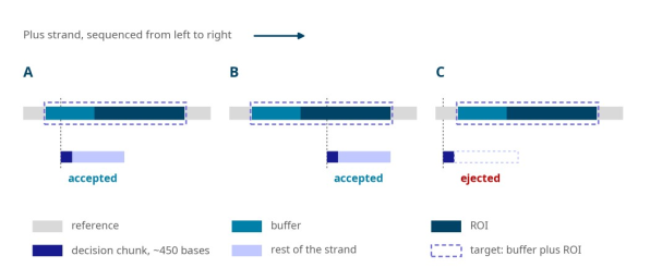
Figure 20: The Adaptive Sampling decision for strands read from the plus strand. The upper lane of each case is the reference with a target made up of its buffer and ROI. (A) A strand which begins inside the buffer is accepted and reads into the ROI. (B) A strand which begins inside the ROI is accepted. (C) A strand which begins upstream of the buffer is ejected once its first chunk has aligned outside the target, and the part of the ROI it would have covered is lost.
31. Buffers, targets and footprint
The decision is made only on the first 450 bases or so. A strand is judged by the position at which it begins, not by the sequence it contains. A strand which begins 10 kb upstream of your ROI and which would go on to sequence through the whole of it, will be rejected unless the buffer covers the position at which it started. This is the entire rationale for defining buffer regions. Defining buffer regions correctly is one of the most important tasks to carry out before starting an Adaptive Sampling run.
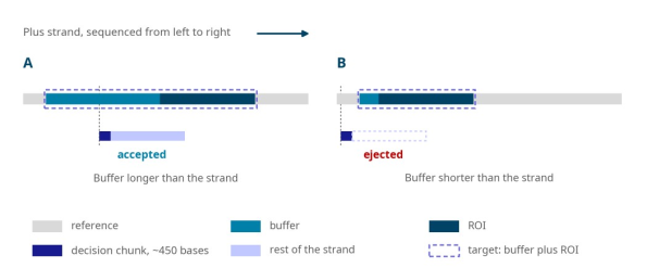
Figure 21: A well-defined buffer region (A) and a badly-defined buffer region (B). In B, the buffer is shorter than the strands in the library. Therefore, strands which would have sequenced through the ROI, begin outside the target and are ejected.
Sizing the buffer
The buffer size should be defined from the read length distribution of your library. It is not possible to know the length of a strand until it has been sequenced in full, but the distribution tells you what to expect. As a guideline, a value between the N25 and the N10 of the distribution is a good measure of the buffer to add to the 5′ end of each target on the plus and minus strands.
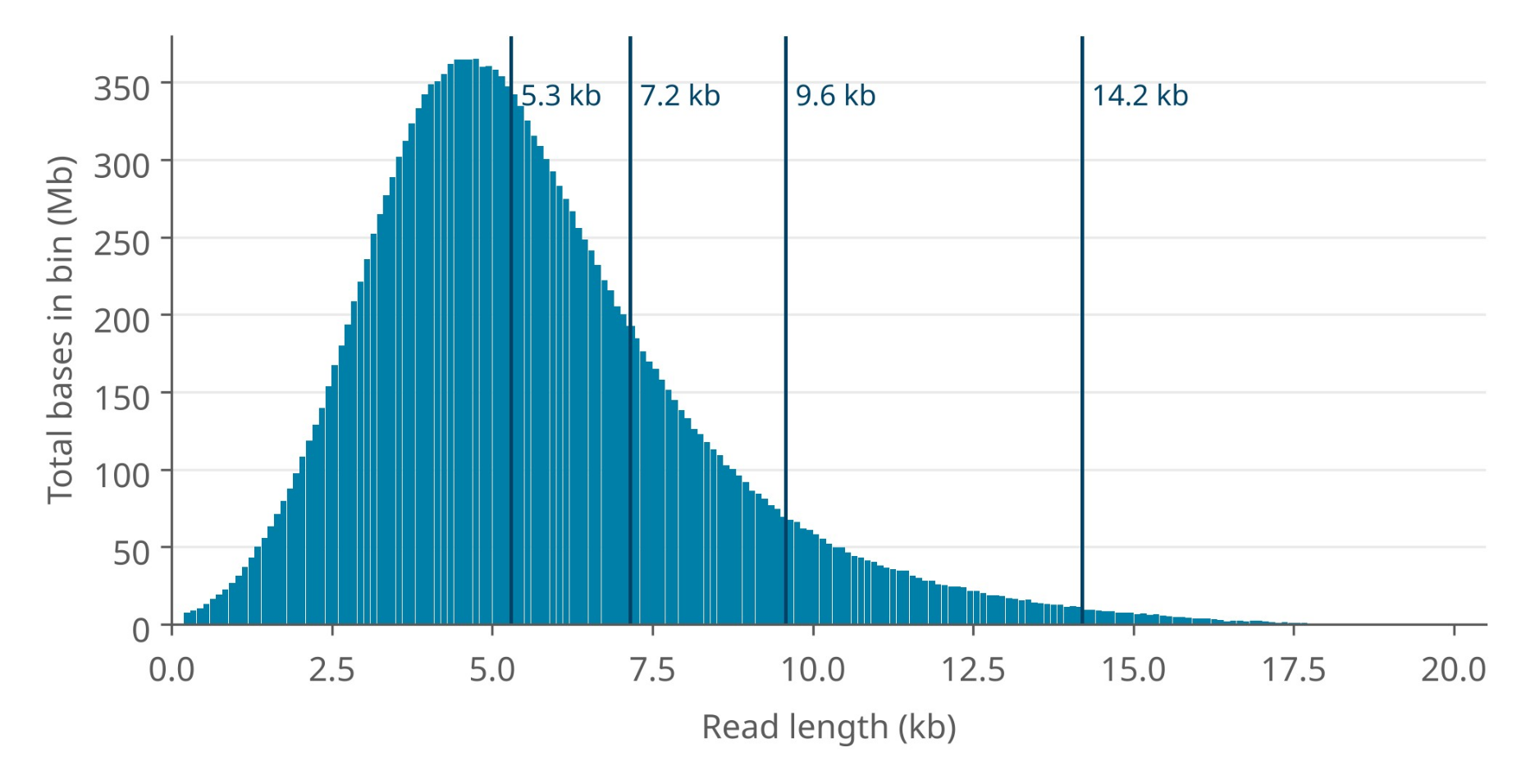
Figure 22: Read length distribution of a 5 kb library fragmented with a Covaris g-TUBE. The vertical lines are the N50, N25, N10 and N01 of the distribution, from left to right.
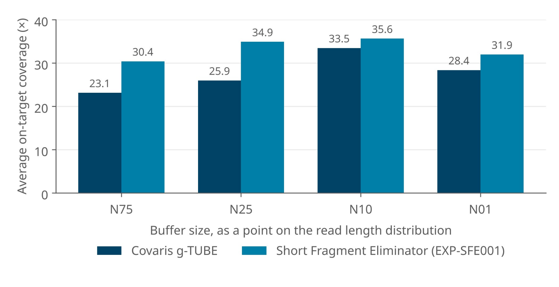
Figure 23: Average on-target coverage obtained from libraries buffered at the N75, N25, N10 and N01 of the read length distribution for a Covaris g-TUBE sheared library and a library prepared with the Short Fragment Eliminator Kit (EXP-SFE001).
The cost of buffer
As buffer is added to each region individually, the cost of a given buffer in footprint scales with the number of regions rather than with the size of the ROIs. The following equation is used to calculate the final target amount for an Adaptive Sampling decision:
Selection target on each strand (bases) = number of targets × Nxx + total ROI bases
With buffer at the 5′ end of each target on the plus and minus strands, as the Digital Panel Designer applies it, each strand selects one buffer length for each target.
Consider two panels, both defined against the 3.2 Gb human genome. In the first, a panel with a small number of large targets, buffer is inexpensive: even a buffer of N01 brings the panel only to 0.68% of the genome. In this case, you should use the largest buffer available to you, since it costs almost nothing in footprint and maximises the chance of capturing a strand which extends into the target.
In the second, a panel with a large number of small targets, buffer dominates. A panel which occupies 4.5% of the genome as ROI alone reaches ~12.5% once an N01 buffer has been added to the 5′ end of the plus and minus strands, which is well beyond the point at which Adaptive Sampling is able to support. Such a high amount of target decreases the enrichment power of Adaptive Sampling by keeping the pores occupied sequencing off-target reads. In this case, reduce the buffer to an N50 or shear the library shorter so that every Nxx value taken from the distribution falls.
Neighbouring targets
The Digital Panel Designer writes two rows for every target, one for each strand, and it does not merge rows belonging to different targets. A buffer is shortened only where it would run into the body of a target which does not already overlap its own, so that it stops at the start of that target. Where two targets overlap or one contains the other, both buffers are added in full. A buffer is also clamped at the start and end of the contig. Where two targets abut exactly, with no gap between them, they are treated as a single region, and the buffer is measured from the outer edge of that region. Figure 24 shows each of these cases.
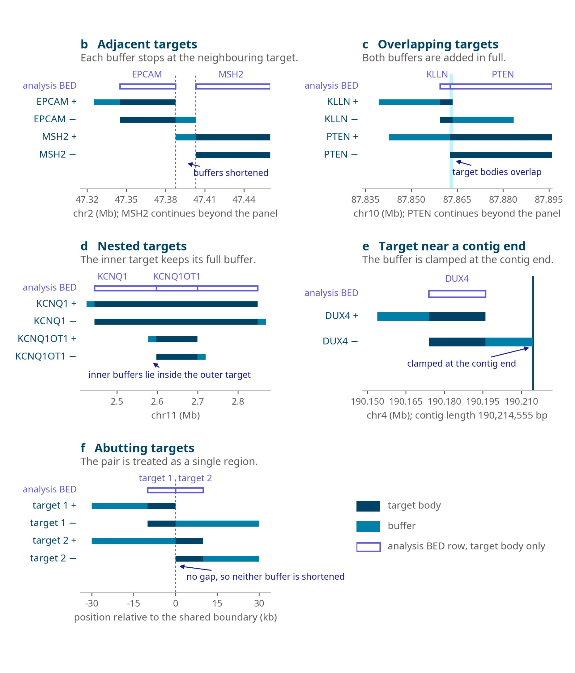
Figure 24: Buffer applied to neighbouring targets at the default of 20 kb. (b) Adjacent targets where each buffer stops at the neighbouring target. (c) Overlapping targets and (d) nested targets where both buffers are added in full. (e) A target near the end of a contig where the buffer is clamped at the contig end. (f) Abutting targets which are treated as a single region.
Minimum coverage versus average coverage
Buffer also has the effect of evening out the coverage obtained within an ROI by allowing the capture of long reads which overlap the ROI only at their very end. A simulation run over 60 different conditions shows the difference between minimum and average coverage narrowing as the buffer increases (Figure 25). You may therefore wish to accept a slightly lower average coverage in favour of a more homogeneous coverage within each ROI, which is often the right choice where variant calling is required across the whole of a region.
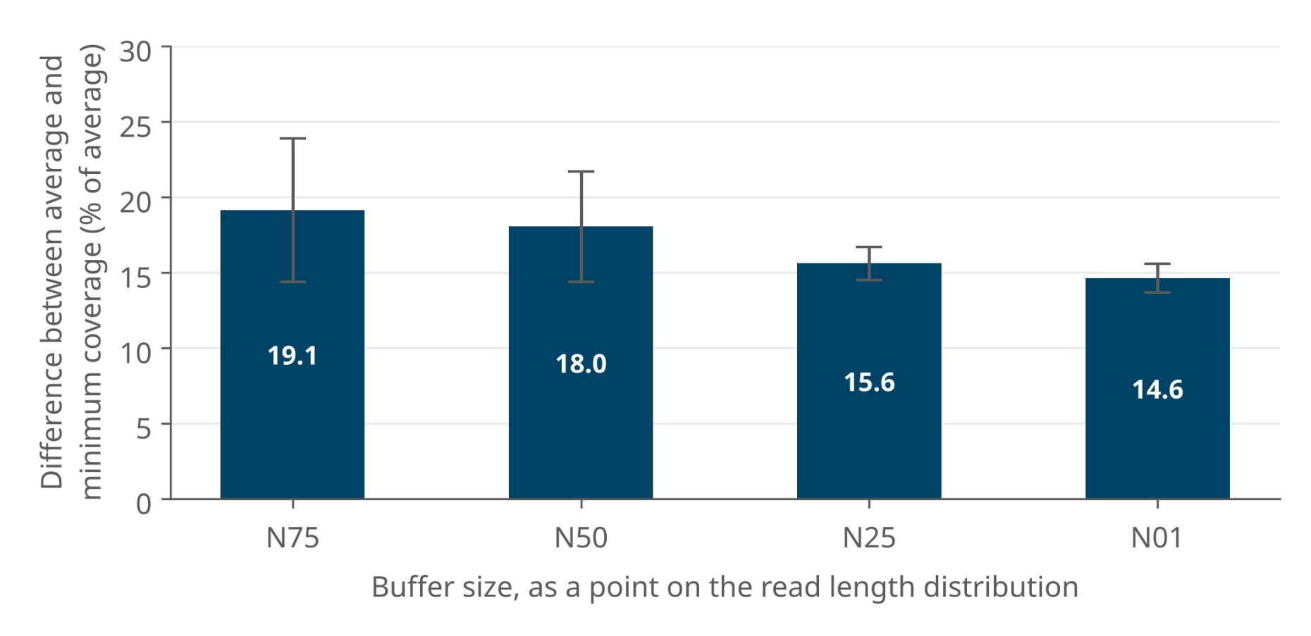
Figure 25: Simulated data showing the difference between the minimum and the average coverage of a region (expressed as a percentage of average coverage) as buffer is increased.
32. Library length
Assuming correctly defined buffers, the benefit obtained each time a strand is rejected is the amount of sample sequenced through in the process. If the strands in your library average 1,000 bases, then each rejection has sampled 1,000 bases of the sample, whereas if they average 30 kb, each rejection has sampled 30 kb. Since the time taken to reach a decision and reject is the same for short and long libraries, a longer library samples the full genome considerably quicker, which matters when the targets are sparse.
In contrast, every acceptance occupies the pore for the full length of the strand. Sequencing 30 kb at 450 bases per second takes ~67 seconds and with a decision time of approximately 1 second, that is around 67 reads which the software could have sampled through instead.
Which of these effects dominates depends on the density of your targets. If your BED file contains 20,000 targets with an average size of 3 kb, the total target is 60 Mb, which corresponds to approximately 2% of the human genome and therefore, to a probability of finding your target in 1 out of every 50 reads sequenced. Sequencing a single 30 kb strand recovers only 3 kb of it. This prevents you from sampling 38 of the 50 reads you need, to find the next on-target read. A 30 kb library used in this situation is detrimental to both enrichment and total coverage.
A better use case would be to target, for example, 200 individual regions with an average of 60 kb per target. A library sheared with the Covaris g-TUBE, giving an N50 of approximately 6 to 8 kb, would be ideal for maximising output while minimising pore blocking and wasted sequencing. Adding a buffer of approximately 20 kb, corresponding to the N01 of that library, would minimise the difference between the average and minimum coverage.
Longer libraries also require a higher mass of input to load the necessary molarity. They block the pores more frequently and require more frequent flow cell washes. Longer libraries may generate a lower total amount of data and the chance of terminal pore blocking is higher for these libraries. However, what they provide in return is faster sampling power and the ability to phase across the regions being targeted.
33. Strand directionality
The Digital Panel Designer applies strand directionality to every panel by default, adding buffer to the 5′ end of each ROI on both the plus and the minus strands. This section describes the mechanism and how to reproduce it in a BED file built by hand as described in Appendix A.
The sixth column of a BED file carries the direction of a sequence. By providing it, you are telling MinKNOW that you are interested in that sequence from one of the strands only. A full stop in the sixth column expresses that you are interested in both strands. Duplicating a region with opposing signs in the sixth column targets the sequence on both strands explicitly.
The principal use of the feature is side-specific buffering, in which buffer is added only upstream of the target on each strand. This prevents acquisition of reads that start downstream of the ROI. It also halves the amount of buffer sequence added. The buffer is applied to a single side of the target on each strand, not indiscriminately to both. To do this, include two lines in the BED file for the same target, one for each strand direction:
chr1   start-buffer   end            name   score   +
chr1   start          end+buffer     name   score   -
Note that reads which start within the ROI will still extend beyond the end of it, since the cut-off applies to the position at which a read begins.

Figure 26: IGV plot coloured by strand direction, showing the effect of strand-specific targeting using the sixth column of the BED file. Coverage falls away on the side of each ROI from which strands were not accepted.
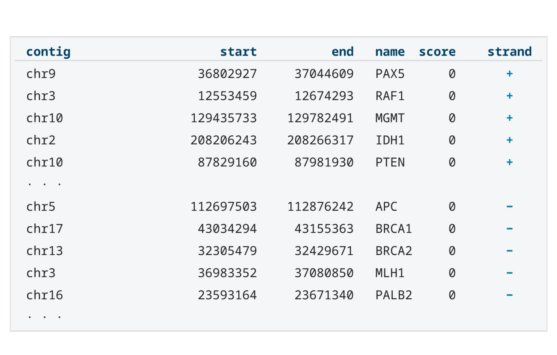
Figure 27: Example of a BED file containing six columns: contig, start coordinate, end coordinate, region name, score, and strand.
Further information is available from the BED specification.
34. Depletion mode
In contrast to running Adaptive Sampling in enrichment mode, in depletion mode you are choosing which sequences to reject rather than which to accept, and this requires a different approach.
The first difference is that the advised total targeted amount is the inverse of what you would use for an enrichment strategy. The amount of sample you specify for rejection needs to be large enough so that the pores have the maximum time available in which to sequence the regions of interest. You can still reach a similar level of enrichment to the enrichment strategy if your sequences of interest comprise a small proportion of the sample, between 1 and 5%. You will need to create a BED file that rejects 95 to 99% of it.
The second difference is that the buffer size needs to work as a negative value when depleting regions from a single genome. Instead of adding buffer to the regions named in the file, you subtract it. The boundary being protected is the edge of the region you wish to keep. It is not the edge of the region you are rejecting. Building a depletion BED file therefore means covering the complement of your ROIs, running from the end of one region to the start of the next and out to the ends of each chromosome, so you will need to know the contig lengths for the reference you are using. These values may vary depending on the reference.
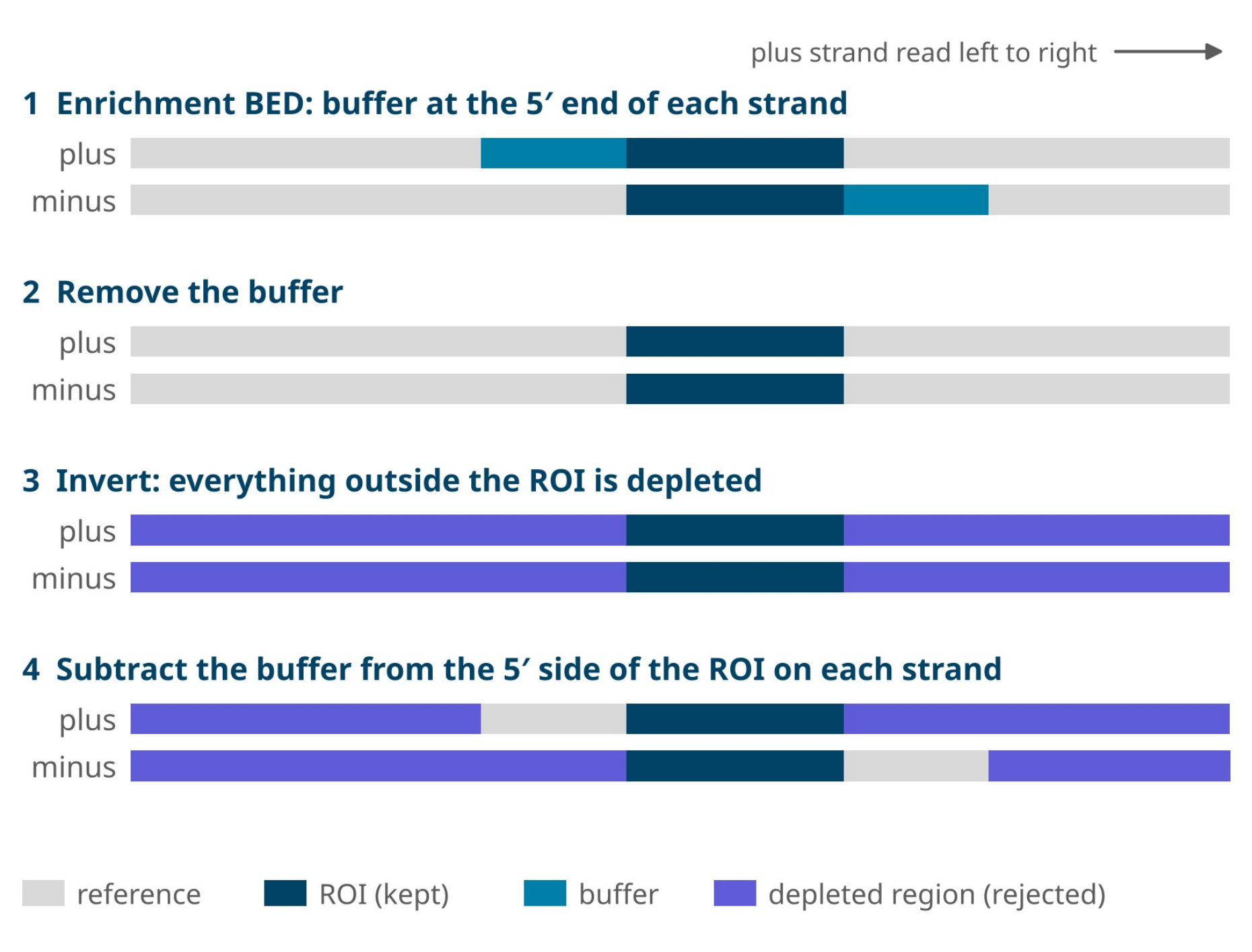
Figure 28: Converting an enrichment BED file into a depletion BED file. The buffer is removed and the regions outside the ROI are inverted into depleted regions. Buffer is then subtracted from the depleted region on the 5′ side of the ROI on each strand, so that strands which start in the buffer and read towards the ROI are not rejected.
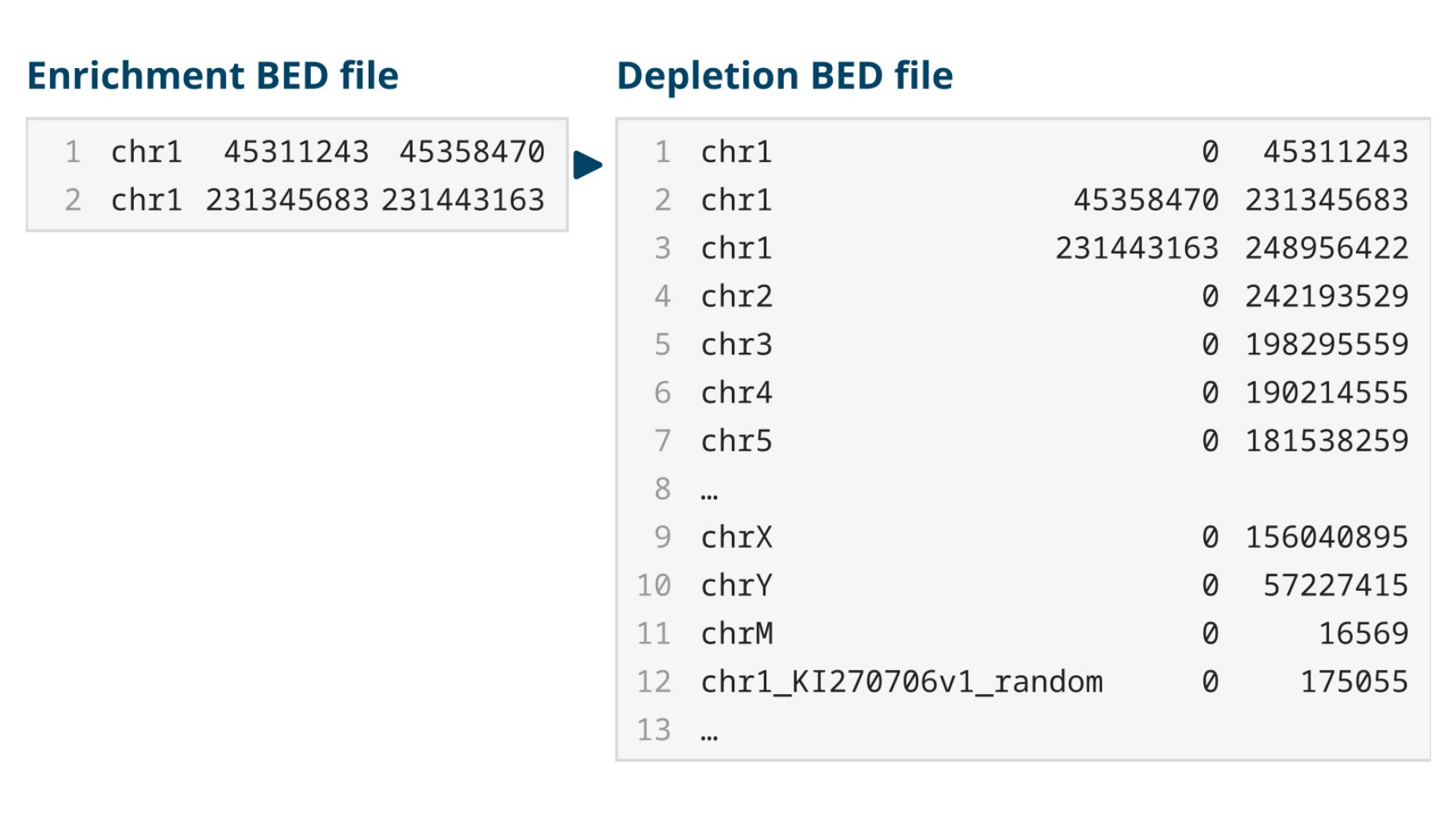
Figure 29: Example of a BED file converted from an enrichment to a depletion strategy. The two enrichment intervals become one interval per contig, split around the regions to be kept. No buffer is applied in this example.
If you are trying to enrich for specific regions by depleting the rest of the sample, it is easier to set up an enrichment strategy instead. Depletion mode is best used when you want to enrich for unknown sequences or genomes. This applies most commonly where a sample contains a mixture of organisms and you wish to deplete everything already known to be present. Adaptive Sampling then enriches whatever rare or unknown genomes that remain.
35. Device limits
Adaptive Sampling requires a great deal of computing power. It basecalls, aligns and reaches a decision on every strand captured in real-time. Anything else running on the device competes with it for these resources.
Live basecalling can run alongside Adaptive Sampling, provided the number of flow cells and the basecalling model stay within the limits of the device given. Using Basecall on-target reads only (BOTO), described in section 22, raises the number of flow cells you can run. Above those limits, decisions slow down, enrichment falls, and on-target coverage is reduced. For the same reason, we recommend that nothing else is running on the device, including offline basecalling, basecalling from whole-genome sequencing runs, and any other process which consumes CPU or GPU resources.
Maximum number of flow cells when running Adaptive Sampling, by basecalling model and setting is listed below:
| Basecalling | Alignment | P24, HAC | P24, SUP | P2i, HAC | P2i, SUP |
|---|---|---|---|---|---|
| All reads | Off | 24 | 11 | 2 | 2 |
| All reads | On | 16 | 7 | 2 | 1 |
| All reads + 5mC/5hmC | Off | 16 | 7 | 2 | 1 |
| All reads + 5mC/5hmC | On | 16 | 7 | 2 | 1 |
| BOTO | Off | 24 | 24 | 2 | 2 |
| BOTO | On | 24 | 24 | 2 | 2 |
| BOTO + 5mC/5hmC | On | 24 | 24 | 2 | 2 |
P24: PromethION 24 P2i: PromethION 2 Integrated
All reads means every strand is basecalled, including rejected strands.
BOTO (Basecall on-target reads only) basecalls accepted strands only.
Alignment refers to the live alignment output option in MinKNOW; Adaptive Sampling always aligns strands to make its decisions.
Methylation calling in CpG or all contexts gives the same limits.
Limits apply to MinKNOW 26.01 and may change in later releases.
Alignment and memory limit
Alignment time is a further consideration, since the larger the reference provided, the longer the Adaptive Sampling process takes to search the indexed reference for the alignment.
As stated in section 5, do not pre-index reference files before uploading them to MinKNOW.
36. Appendix A — designing a panel without the Digital Panel Designer
This appendix describes the manual route for cases that the Digital Panel Designer does not cover: an organism with no gene model in Ensembl or NCBI, classes of annotation which the tool does not resolve, or a machine with no network access. For every other panel, refer to the section on the Digital Panel Designer.
Reference and BED file
Reference FASTA files can be downloaded from trustworthy databases such as the UCSC Table Browser and the NCBI RefSeq database. The most important point to consider is that the reference used for the sequencing run must be the same reference which was used to produce the annotation your coordinates came from. A BED file built against one assembly and run against another will produce a run which works but which targets the wrong sequence.
If more than one organism is present in the sample, download a reference for each and concatenate the files, checking first that no contig name is duplicated between them.
To build a BED file from a UCSC Table Browser annotation (Figure 30):
Select the clade, genome and assembly.
Select a group. The group corresponds to the type of sequence you are targeting, for example, genes and gene predictions, regulation sequences or regions of structural variation. It determines the tracks which are available to you.
Select a track and a table. The table gives the list of regions provided by that track.
Under Define region of interest, either select genome to retrieve the whole genome or enter an interval of coordinates and click lookup to activate the selection.
Under Retrieve and display data, set the output format to BED - browser extensible data, enter a file name and set the file type returned to plain text. MinKNOW does not accept compressed files.
Click get output.
On the page which follows (Figure 32), ensure that Include custom track header is not selected.
Under Create one BED record per:, select Whole Gene. This gives you the exact regions defined in the track. Other options are available if you are interested in upstream, downstream or strand-specific sequence only.
Click get BED. The file will download without an extension. Rename it to name_chosen.bed.

Figure 30: Table Browser settings for downloading a BED file of common structural variation regions on the human X chromosome.

Figure 31: The list of tables in the dbVar Common SV track.

Figure 32: The last page in the Table Browser before the BED file is downloaded.
The file produced by this procedure does not contain buffer. Buffer is added with bedtools slop as described below.
Manual buffer configuration
You will need samtools and bedtools installed on your computer. This may require some previous knowledge of how to use Conda, samtools and bedtools.
Set up an environment, if you do not already have one:
wget https://repo.anaconda.com/miniconda/Miniconda3-latest-Linux-x86_64.sh
bash Miniconda3-latest-Linux-x86_64.sh -b -f -p
source ~/miniconda3/bin/activate
conda create --name adasamp -c bioconda samtools bedtools
conda activate adasamp
Navigate to the folder containing your FASTA and BED files. If they are in different folders, create a link to the location of the other file with ln -s:
REF=your_reference.fasta
BED=your_bed_with_target_regions.bed
BASES_TO_EXPAND_PER_SIDE=20000
The buffer size determined in section 31:
CHROM_SIZES=${REF}.chrom.sizes SLOPPED_BED=${BED%.*}_slop-${BASES_TO_EXPAND_PER_SIDE}.bed
Index the reference and obtain the chromosome sizes, so that slop can clamp at contig ends:
samtools faidx ${REF}
cut -f1,2 ${REF}.fai > ${CHROM_SIZES}
Expand the BED file by the buffer amount on each side of every region:
bedtools slop -l ${BASES_TO_EXPAND_PER_SIDE} -r ${BASES_TO_EXPAND_PER_SIDE} \ -i ${BED} -g ${CHROM_SIZES} > ${SLOPPED_BED}
These commands take the BED file containing your regions of interest and adds a number of bases on either side of each ROI, which is the buffer region for the Adaptive Sampling selection. The intermediate files are saved in the location from which the commands are run and will remain there until deleted.
These commands add buffer to both sides of each ROI. The Digital Panel Designer adds buffer only to the 5′ end of each ROI on the plus and minus strands, as described in section 33. To reproduce this, use the following commands in place of bedtools slop above. The first command writes each ROI twice, once for each strand, and the second adds the buffer upstream of each row according to its strand, clamping at the ends of each contig.
STRANDED_BED=${BED%.*}_stranded.bed
Write each ROI, once for each strand:
awk 'BEGIN{OFS="\t"} {n=($4=="")?".":$4; print $1,$2,$3,n,0,"+"; print $1,$2,$3,n,0,"-"}' \
${BED} > ${STRANDED_BED}
Add the buffer upstream of each row, according to its strand:
bedtools slop -s -l ${BASES_TO_EXPAND_PER_SIDE} -r 0 \ -i ${STRANDED_BED} -g ${CHROM_SIZES} > ${SLOPPED_BED}
${SLOPPED_BED} is the file to load under Adaptive Sampling in MinKNOW and the original unbuffered ${BED} is the file to load under Alignment, as described in section 21.
37. Appendix B — output files and field definitions
The files which MinKNOW outputs during a sequencing experiment are described in the Data analysis technical document. For Adaptive Sampling experiments, there are two additional CSV files saved in the adaptive_sampling folder within the run folder, which can be used for troubleshooting. Either file can be matched to the sequencing summary by read_id which allows you to see the metrics for each read alongside the decision Adaptive Sampling made about it.
AS_decisions_x_x_x.csv
| Field | Description |
|---|---|
| read_id | An individual ID for each read, matching the read IDs provided by the sequencing summary. |
| action | Whether a read was accepted (sequence) or rejected (unblock) |
| action_response | Whether the action was successfully executed by MinKNOW (SUCCESS, FAILED_READ_FINISHED or FAILED_READ_TOO_LONG) |
AS_timings_x_x_x.csv
| Field | Description |
|---|---|
| channel | The channel in which the read was sequenced. |
| read_id | As above |
| batch_time | Batch time of when the read was processed by the Adaptive Sampling script. |
| samples | Number of samples received by the Adaptive Sampling script for each read. |
| bases | Number of bases basecalled from each read for the Adaptive Sampling decision. |
| barcode_arrangement | Barcode arrangement detected on the first chunk. This will be empty if you are not using a barcoding kit. |
| mean_qscore | Mean Q-score of the Adaptive Sampling first chunk basecalling. |
| time_to_package_and_send | Time between the Adaptive Sampling script receiving a read and sending it to the basecaller. |
| time_in_basecaller | Time between sending a read to the basecaller and receiving it back. |
The run-level summary is held in adaptive_sampling.csv, in the other reports folder.
38. Digital Panel Designer — frequently asked questions
A list of FAQs is listed below.
39. The tool
What is the Digital Panel Designer?
The Digital Panel Designer is a browser-based tool for building the digital panel used by Adaptive Sampling. You give it the regions you want to enrich and it returns a set of interval files in BED format which MinKNOW and your downstream analysis can read. A digital panel is defined in software, not in chemistry, so it can be changed between runs at no cost and with no change to the library preparation.
Does it design depletion panels as well as enrichment panels?
The tool is built around enrichment, where the regions you supply are the regions you keep. Depletion inverts that relationship and a depletion panel is usually a small number of very large intervals, whereas an enrichment panel is many small ones. Section 34 of this guide describes how to construct one.
40. References and targets
Which reference assemblies can I design against?
GRCh38 and GRCh37 are offered for human in this release, and we expect to add more genomes in future releases. The assembly is chosen first, before any targets are added, and every coordinate in the panel is resolved against it.
Can I design a panel for a non-human genome?
Not in this release. Please follow the manual design instructions in Appendix A (section 36) or contact Tech Support.
How do I add my targets?
There are four routes and you can use more than one of them in the same panel. Select one of the ready-to-use panels from the preset list, type or paste gene names, enter coordinates directly, or upload an existing BED file. Whichever route you use, the rows arrive in the same target table and are treated identically from that point on.
Which gene names does it accept?
Use HGNC approved symbols wherever you have them, and each name is then looked up in Ensembl first. A name filed under another symbol is resolved through HGNC and then the Ensembl gene identifier, and NCBI Gene is consulted last. The table records which service placed each row.
Why do the coordinates differ from the ones I already had for a gene?
RefSeq and Ensembl place some gene models differently. For genes which both services know, the two sets of coordinates can disagree by as much as a few kilobases. The source column in the target table tells you which one placed each row. The disagreement is genuine, and it is not resolved by either service. We recommend reviewing it before you export.
In what format do I enter coordinates?
Enter one region per line, in the form chr17:43,044,295-43,170,245. Commas are optional. Use the These coordinates are dropdown to state how your coordinates are written: 0-based, half-open (BED), which is the default, or 1-based, inclusive, as shown in IGV, the UCSC Genome Browser and Ensembl. The exported BED files are always 0-based.
How many targets can a panel contain?
There is no fixed limit on the number of targets. The limit which matters is the footprint of the finished panel, which is the total length of sequence the panel occupies once buffer has been added. Panels of well over a thousand genes are workable where the footprint stays within range; section 11 covers the footprint limits.
What are the ready-to-use panels?
Four research-use-only panels are supplied with the tool, and each one can be loaded from the preset list in a single step.
| Digital panel | Research application | Targets | Sequencing protocol |
|---|---|---|---|
| Hereditary Cancer | Cancer predisposition | 258 genes (259 targets) | Multiplex |
| Pharmacogenomics | Drug response | 375 genes | Multiplex |
| Pan-Cancer | Tumour profiling | 723 genes | Singleplex or Ultra-rapid singleplex |
| Pan-Haematological Cancer | Haematological malignancies | 144 genes | Singleplex |
Can I edit a ready-to-use panel?
Yes, a preset is a starting point and not a fixed list. Once loaded, its rows can be removed and your own targets added alongside them, and the buffer applies to the whole panel in the usual way.
41. Buffer and footprint
What is buffer and why does the tool add it?
Buffer is flanking sequence added to the 5′ end of every region of interest on both the plus and minus strands. The Adaptive Sampling decision is made on the first 450 bases or so of a strand and a strand which begins a few kilobases upstream of your region is rejected before the region is reached. Buffer brings those upstream start positions inside the panel, and the strands which begin there are then accepted and sequenced through into your region.
What buffer does the tool apply and can I change it?
The default is 20 kb at the 5′ end of each target on the plus and minus strands, and you can adjust it anywhere between 10 kb and 30 kb, in steps of 1 kb. The footprint readout then updates as you move the control.
How do I choose a value?
Take the value from the read length distribution of your library. A value between the N25 and the N10 of that distribution is a good starting point; longer libraries need more buffer. Where a long library drives the footprint out of range, shearing the library shorter is often a better solution than reducing the buffer.
My footprint is much larger than the total length of my regions. Why?
Buffer is added to each region individually. Therefore, every region carries twice the buffer value in addition to its own length. A panel of 200 small regions with a 20 kb buffer occupies around 8 Mb before the regions themselves are counted. The more regions a panel contains, the more a given buffer costs.
What happens where two targets are close together?
Their buffers meet and the tool merges the two into a single region. Adaptive Sampling would merge the two targets in any case. The reported footprint reflects the merged length and does not count the overlap twice.
What happens at the start and end of a chromosome?
Buffer is clamped at the ends of each contig. A target lying near a telomere or a target on a short contig (such as the mitochondrial genome) receives as much buffer as the contig is able to provide and no more.
42. Checks and warnings
Why is the tool warning me about my mitochondrial target?
The mitochondrial genome is around 16.6 kb long, which is shorter than the default buffer. Once the buffer is clamped to the ends of the contig, the target covers the whole of it. The warning tells you that the buffer you asked for could not be applied in full but the panel is still valid and can be exported.
Why can I not export my panel?
Export is prevented where the footprint falls below 0.1% of the genome or rises above 10%. The lower limit catches panels too small to enrich usefully and the upper limit catches panels large enough that Adaptive Sampling will not improve on a standard sequencing run. Both are design-time safeguards, and the device does not impose these.
Does the tool check my panel for design problems?
Yes, the checks are of two kinds. A blocking check stops the export and produces no files. Both blocking checks are related to the size of the panel.
A warning appears in the panel summary against the target it concerns, but a warning never stops the export. It tells you that the panel will behave differently from the way it reads and each one needs a decision from you.
These two conditions stop the export:
| Condition | What happens |
|---|---|
| Footprint below 0.1% of the genome | Export is prevented. Refer to Why can I not export my panel? above. |
| Footprint above 10% of the genome | Export is prevented. Refer to Why can I not export my panel? above. |
These conditions raise a warning and leave a valid panel which exports normally:
| Warning | What it means | What to do |
|---|---|---|
| The buffer was clamped at the end of a contig. | The target lies close to the end of a chromosome or on a short contig, such as the mitochondrial genome, and the full buffer would run past the end of the sequence. The tool applies as much buffer as the contig allows. | Nothing. The panel is valid and the geometry is correct. Refer to Why is the tool warning me about my mitochondrial target? above. |
| The gene name matched more than one gene record. | The name you entered appears more than once in the annotation, and the tool has taken one record and set the others aside. | Check the coordinates on that row in the target table and enter the coordinates directly where the record taken is not the one you meant. |
| The target has a near-identical copy elsewhere in the genome. | A paralogue that shares enough sequence with your target that reads from either copy can be placed on the other, and measured coverage on the target can then read high or low. | Decide whether to add the second copy to the panel. The tool does not add it for you. |
43. Exported files and MinKNOW
What do I get when I export?
Three interval files are produced:
| File | Contents | Where it is used |
|---|---|---|
| *_enrichment.bed | Regions plus buffer, merged | MinKNOW, the Adaptive Sampling BED field |
| *_analysis.bed | Regions only, without buffer | Secondary analysis |
| *_exons.bed | Exon-level intervals | Downstream coverage analysis. Not loaded into MinKNOW |
Which file do I load into MinKNOW?
Load *_enrichment.bed into the Adaptive Sampling BED field, as this is the only file that MinKNOW uses to make decisions. Loading the unbuffered file instead will affect enrichment, as strands which begin upstream of your regions will then be rejected.
What is the unbuffered file for?
Use *_analysis.bed after the run for calculating coverage over your regions, for restricting variant calling to them, and for any other step which requires your targets alone, without their flanking sequence. It is not a sequencing input.
The names in my exported file are not the names I entered.
Rows added by coordinates or by BED upload are given a generated name where none were supplied.
44. Performance and support
What enrichment should I expect?
This depends on the footprint of your panel and on your library. In the Hereditary Cancer Panel application, the targeted genes reached 36 to 65x coverage while the rest of the genome was covered 3 to 5x in the same run. A panel with a footprint below approximately 5% of the genome is comfortable. Above this figure, enrichment begins to fall away, as the pores spend an increasing proportion of the run sequencing accepted flanking sequence.
Will a smaller panel give me deeper coverage of my targets?
Not reliably and not in proportion. Reducing a panel from 5% of the genome to 1% does not multiply your on-target depth by five. Yield per flow cell, library length and pore occupancy set the upper limits, and the footprint sets how much of that yield lands on your targets. Design the panel around the regions you need rather than around a footprint target.
Which devices should I use?
The protocols are optimised for PromethION. PromethION 2 Integrated and PromethION 24 are recommended for Adaptive Sampling. Adaptive Sampling is computationally demanding as every strand is basecalled and aligned in real-time. The number of flow cells a device can run simultaneously depends on the basecalling model in use (refer to section 35, Device limits).
Do I lose the data from the rejected strands?
No, rejected strands are still sequenced for the first few hundred bases and those reads are written to the run folder. They give a low-pass view of the rest of the genome alongside your targeted data, and where the library was prepared from native DNA, the base modifications are called in the same run.
Can I change the panel part way through a run?
No, the panel is read when the run starts. To change targets, you should stop the run and start a new one with the new BED file or plan the change as a separate run.


