Adaptive Sampling is a method for digital target enrichment unique to Oxford Nanopore Technologies. It uses a digital panel defined by the genomic coordinates of the target regions of interest (e.g. genes and promoter regions) provided in BED format. During sequencing, a BED file containing these target regions with additional sequence padding is used to guide enrichment. For downstream analyses, such as target enrichment, coverage assessment, and variant calling, a separate BED file is required that contains the original target regions without padding.

This guide provides an overview of methods for bioinformatic analyses of Adaptive Sampling tumour-only experiments, with a particular focus on methylation profiling and variant analysis. A reduced set of the same analysis tools can be used for the analysis of shallow whole genome experiments.

The methods described within this guide are provided as examples of bioinformatic analyses that may be performed on Adaptive Sampling data. These methods are provided for research use only and on an as-is basis, without any representation, warranty, or guarantee of performance, suitability, or fitness for a particular purpose.

To find out more about Adaptive Sampling, visit our Adaptive Sampling and digital panels page.

Variant calling

We recommend using Oxford Nanopore Super Accurate (SUP) basecalling model with methylation enabled for single nucleotide variant (SNV) calling, as it provides the best available accuracy for variant detection. However, this benefit does not extend to copy number alteration (CNA) or structural variant (SV) analyses for which either High Accuracy (HAC) or SUP v5.2 basecalling models provide similar performance.

Somatic SNV calling from tumour-only Adaptive Sampling datasets is restricted to the target-only regions defined in the target BED file (no padding, no strand specificity) that was used to define the Adaptive Sampling targets.

• Use Dorado V1.3.3 and SUP basecalling with model generations 5.0 and above (e.g. MinKNOW 26.0).

• We recommend at least 100x on-target coverage as the preferred setup.

• Approximately 75x on-target mean coverage may be sufficient, but sensitivity for lower variant allele frequency (<10% VAF) variants is expected to be reduced.

• Use GRCh38 as the reference genome and run variant calling in BED-restricted tumour-only mode using an Adaptive Sampling target BED file (no padding, no strand specificity).

• DeepSomatic is the recommended method when recovery of lower VAF variants (≤10% VAF) is the main priority. We have tested v1.9.0.

• ClairS-TO is the balanced alternative and generally carries a lower false positive burden. We have tested v0.4.0.

• ClairS-TO

• DeepSomatic

• Aligned reads: Tumour BAM or CRAM aligned to GRCh38, with index

• Reference genome: GRCh38 reference FASTA and associated index files.
  We recommend:

  • for the ONT_AS_PanCancer V1: GRCh38_GIABv3_no _alt_analysis_set_maskedGRC_decoys_MAP2K3_KMT2C_KCNJ18.fasta.gz
  • for the ONT_AS_PanHaem V1: GCA_000001405.15_GRCh38_no_alt_analysis_set.fna

• Target regions: Adaptive Sampling target BED

• Container software: Apptainer installed on the analysis system

ClairS-TO

Install Apptainer, then pull a ClairS-TO container image:

apptainer pull clairs-to.sif docker://hkubal/clairs-to:latest

Verify the installation:

apptainer exec clairs-to.sif /opt/bin/run_clairs_to --help

DeepSomatic

Install Apptainer, then pull a DeepSomatic container image:

apptainer pull deepsomatic.sif 
docker://google/deepsomatic:latest

Verify the installation:

apptainer exec deepsomatic.sif run_deepsomatic --help

Example inputs

• Aligned reads: /abs/path/input/tumour.sup.on_target.bam

• Index file for aligned reads: /abs/path/input/tumour.sup.on_target.bam.bai

• Reference genome: /abs/path/input/GRCh38.fa

• Index file for reference genome: /abs/path/input/GRCh38.fa.fai

• Target regions (analysis BED file): /abs/path/input/adaptive_sampling_targets.bed

• Desired output directory: /abs/path/output/

Example run: small somatic variant calling with ClairS-TO

The example below shows a tumour-only analysis restricted to regions specified in a BED file, using Oxford Nanopore sequencing data that was basecalled with Dorado using the SUP model.

INPUT_DIR=/abs/path/input
OUTPUT_DIR=/abs/path/output/clairs_to
THREADS=8

mkdir -p "${OUTPUT_DIR}" apptainer exec \
 -B "${INPUT_DIR}:${INPUT_DIR}" \
 -B "${OUTPUT_DIR}:${OUTPUT_DIR}" \
 clairs-to.sif \
 /opt/bin/run_clairs_to \
--tumor_bam_fn "${INPUT_DIR}/tumour.sup.on_target.bam" \
--ref_fn "${INPUT_DIR}/GRCh38.fa" \
--threads "${THREADS}" \
--platform ont_r10_dorado_sup_5khz_ssrs \
--bed_fn "${INPUT_DIR}/adaptive_sampling_targets.bed" \
--output_dir "${OUTPUT_DIR}"

Expected ClairS-TO outputs

clairs_to/ 
 snv.vcf.gz                 

Example run: somatic small variant calling with DeepSomatic

The example below shows a tumour-only analysis restricted to regions specified in a BED file.

INPUT_DIR=/abs/path/input
OUTPUT_DIR=/abs/path/output/deepsomatic
THREADS=12

mkdir -p "${OUTPUT_DIR}/logs" "${OUTPUT_DIR}/intermediate_results_dir"
apptainer exec \
 -B "${INPUT_DIR}:${INPUT_DIR}" \
 -B "${OUTPUT_DIR}:${OUTPUT_DIR}" \
 deepsomatic.sif \
 run_deepsomatic \
 --model_type=ONT_TUMOR_ONLY \
 --ref="${INPUT_DIR}/GRCh38.fa" \
 --reads_tumor="${INPUT_DIR}/tumour.sup.on_target.bam" \
 --regions="${INPUT_DIR}/adaptive_sampling_targets.bed" \
 --output_vcf="${OUTPUT_DIR}/somatic.vcf.gz" \
 --sample_name_tumor="SAMPLE_ID" \
 --num_shards="${THREADS}" \
 --logging_dir="${OUTPUT_DIR}/logs" \
 --intermediate_results_dir="${OUTPUT_DIR}/intermediate_results_dir" \
 --use_default_pon_filtering=true \
 --dry_run=false

Expected DeepSomatic outputs

deepsomatic/
 somatic.vcf.gz logs/
 intermediate_results_dir/

Practical Recommendation

If the primary goal is improved detection of lower VAF variants, DeepSomatic should be considered the lead recommendation, with the explicit caveat that it produces more false positives and may require greater downstream variant filtering and review.

If a more balanced SNV callset is preferred, ClairS-TO is an appropriate alternative.

Somatic structural variant calling from tumour-only Adaptive Sampling datasets.

Use the full basecalled BAM (on and off-targets) from the Adaptive Sampling run as input.

Do not restrict structural variant calling to on-target reads only. This is important because structural variant detection depends on collecting enough supporting reads for each event, and one or both breakends may fall outside the Adaptive Sampling target regions. In practice, greater sequencing yield improves the chance of recovering lower variant allele frequency (VAF) of structural variants because when calling breakpoints, the recommended tool Severus, uses a minimum supporting read threshold of 3.

Run Severus in tumour-only mode on the full Adaptive Sampling BAM, aligned to GRCh38. We have tested v1.6.

Use the standard Severus supporting resources, part of the Severus package, for tumour-only calling:

• A panel of normals (PoN)
• A VNTR annotation BED

Severus

Structural variant recovery is strong when Severus is run in tumour-only mode on the full Adaptive Sampling BAM.

The workflow supports recovery of multiple structural variant classes, including translocations, deletions, duplications, and insertions.

In practice, the main sensitivity driver is whether enough supporting reads are present for a breakpoint to pass the minimum supporting read threshold used by Severus.

• Tumour BAM aligned to GRCh38, with BAM index
• PoN file for tumour-only Severus calling
• VNTR BED annotation for GRCh38 – this file helps with regions with higher variability and more challenges in alignment to relax some of the internal thresholds and help process variants.
• Severus installation

The simplest installation method is via conda:

conda create -n severus_env severus conda   
activate severus_env
severus --help

Alternatively, install from source:

git clone https://github.com/KolmogorovLab/Severus
cd Severus
conda env create --name severus_env --file environment.yml
conda activate severus_env
./severus.py --help

Example inputs

• /abs/path/input/tumour.all_minknow_pass.sort.bam
• /abs/path/input/tumour.all_minknow_pass.sort.bam.bai
• /abs/path/input/PoN_1000G_hg38_extended.tsv.gz
• /abs/path/input/human_GRCh38_no_alt_analysis_set.trf.bed
• /abs/path/output/

Example run

The example below shows a tumour-only Severus run on the full Adaptive Sampling BAM.

INPUT_DIR=/abs/path/input
OUTPUT_DIR=/abs/path/output/sample_severus_tonly
THREADS=24

mkdir -p "${OUTPUT_DIR}" severus \
 --target-bam "${INPUT_DIR}/tumour.all_minknow_pass.sort.bam" \
 --PON "${INPUT_DIR}/PoN_1000G_hg38_extended.tsv.gz" \
 --vntr-bed "${INPUT_DIR}/human_GRCh38_no_alt_analysis_set.trf.bed" \
 --out-dir "${OUTPUT_DIR}" \
 -t "${THREADS}"

Expected output structure

sample_severus_tonly/
 breakpoints_double.csv
 read_qual.txt severus.log
 all_SVs/ breakpoint_clusters.tsv
  breakpoint_clusters_list.tsv
  severus_all.vcf
  plots/ severus_0.html
   severus_1.html
   ...
 somatic_SVs/ breakpoint_clusters.tsv
  breakpoint_clusters_list.tsv
  severus_somatic.vcf
  plots/ severus_0.html
   severus_1.html
   ...

Expected key outputs

• all_SVs/severus_all.vcf
• somatic_SVs/severus_somatic.vcf
• all_SVs/breakpoint_clusters.tsv
• somatic_SVs/breakpoint_clusters.tsv
• interactive HTML plots under all_SVs/plots/ and somatic_SVs/plots/
• severus.log for run provenance and troubleshooting

Practical recommendation

For tumour-only Adaptive Sampling SV analysis, use the full basecalled BAM as input and run Severus in tumour-only mode with a PoN and VNTR BED.

The main practical driver of sensitivity is not a single coverage threshold, but whether enough SV-supporting reads are present to pass the minimum supporting read threshold required by Severus.

Large-scale copy number inference from tumour-only Adaptive Sampling data or shallow whole-genome sequencing.

Copy number calling depends on genome-wide coverage, so all reads should be basecalled and retained. It is not sufficient to analyse on-target reads only.

ichorCNA is a good option for large-scale copy number analysis in tumour-only nanopore datasets, provided that genome-wide coverage is available.

ichorCNA

Known or anchored purity mode is the preferred operating mode for complex tumour genomes, because it gives more stable and interpretable copy number solutions.

Free mode can still provide useful broad copy number information however, it is more prone to underestimating tumour purity and compressing copy number amplitude in complex aneuploid samples.

This workflow is most appropriate for broad, large-scale copy number events, including chromosome arm and chromosome scale changes. It should not be presented as a validated workflow for focal copy number alterations.

Note: We recommend using the ichorCNA GitHub repository linked above and v.0.6.0.
There is another repository elsewhere that has an earlier version of the code.

A practical starting point could be 16 hours of sequencing (>2x; >6 Gb of PASS data). For complex whole-genome copy number profiles, 6–8x is a more comfortable operating range. Lower coverage can still provide broad copy number information however, confidence and stability are reduced.

Note that analysis time can still vary depending on parameters like sequencing yield, flow cell performance, sample quality and dataset size.

• Tumour BAM aligned to GRCh38, with BAM index
• Local ichorCNA checkout and installation
• HMMcopy readCounter
• GC wiggle file for GRCh38 at the chosen bin size
• Mappability wiggle file for GRCh38 at the chosen bin size
• GRCh38 centromere annotation file

An example docker/singularity and conda-based setup are shown below.

Container-based usage (recommended)

To avoid R and Bioconductor dependency issues, ichorCNA can be run via the official Docker container.

Note: Container tags (e.g. 3.0.0) do not correspond directly to the ichorCNA R package version (e.g. 0.6.0), but bundle a tested environment.

Docker:

docker pull gavinhalab/ichorcna:3.0.0

docker run --rm -v /abs/path:/data gavinhalab/ichorcna:3.0.0 \
readCounter --help
docker run --rm gavinhalab/ichorcna:3.0.0 \ Rscript /ichorCNA/R/runIchorCNA.R --help

Singularity / Apptainer:

singularity pull ichorcna_3.0.0.sif docker://gavinhalab/ichorcna:3.0.0

singularity exec --bind /abs/path/:/data ichorcna_3.0.0.sif \ readCounter --help

singularity exec --bind /abs/path/:/data ichorcna_3.0.0.sif \
Rscript /ichorCNA/R/runIchorCNA.R --help

Conda:

conda create -n ichorcna_060 \
-c conda-forge -c bioconda \ r-
base=4.4 \
r-remotes r-optparse r-domc r-foreach   
r-ggplot2 r-stringr r-data.table r-plyr r-matrix \                          
bioconductor-hmmcopy \
bioconductor-genomicranges \
bioconductor-genomeinfodb \
bioconductor-delayedarray \
bioconductor-s4arrays \
bioconductor-biostrings \
bioconductor-rsamtools \
bioconductor-rtracklayer \
bioconductor-bsgenome \
bioconductor-bsgenome.hsapiens.ucsc.hg19 \
bioconductor-bsgenome.hsapiens.ucsc.hg38 \
samtools hmmcopy python=3.10 git wget -y

conda activate ichorcna_060

git clone https://github.com/GavinHaLab/ichorCNA.git/abs/path/software/ichorCNA cd /abs/path/software/ichorCNA
git checkout v0.6.0

R -q -e "remotes::install_local('./', dependencies = FALSE, upgrade = 'never')" R -q -e 

"library(ichorCNA); packageVersion('ichorCNA')"

readCounter --help

Rscript ./R/runIchorCNA.R --help

• Known or Anchored Purity Mode

Use when an external purity estimate is available. This is the recommended operating mode for complex tumour genomes, because it gives the most stable and interpretable copy number solution.

• Free Mode

Use when purity is unknown. This can still be informative however, in complex highly aberrant genomes, it often underestimates tumour purity and compresses copy number amplitude, which reduces copy number accuracy.

• /abs/path/input/tumour.all_reads.sort.bam
• /abs/path/input/tumour.all_reads.sort.bam.bai
• /abs/path/software/ichorCNA/
• /abs/path/output/

1. Generate 1 Mbp read-count bins

readCounter --window 1000000 \
 --chromosome "chr1,chr2,chr3,chr4,chr5,chr6,chr7,chr8,chr9,chr10,chr11,chr12,chr13,chr14,chr15,chr16,chr17,chr18,chr19,chr20,chr21,chr22,chrX,chrY" \
 /abs/path/input/tumour.all_reads.sort.bam \
 > /abs/path/output/sample.1000000.wig

2. Run ichorCNA in Known or Anchored Purity Mode

Here, --normal is the normal fraction, not the tumour purity. For example, a sample estimated to be 60% tumour should be run with --normal 0.40

Rscript /abs/path/software/ichorCNA/scripts/runIchorCNA.R \
 --id SAMPLE \
 --WIG /abs/path/output/sample.1000000.wig \
 --gcWig /abs/path/software/ichorCNA/inst/extdata/gc_hg38_1000kb.wig \
 --mapWig /abs/path/software/ichorCNA/inst/extdata/map_hg38_1000kb.wig \
 --centromere \ /abs/path/software/ichorCNA/inst/extdata/GRCh38.GCA_000001405.2_centromere_acen.txt \
 --normal 0.40 \
 --estimateNormal FALSE \
 --ploidy "c(2,2.5,3)" \
 --sex male \
 --normalizeMaleX TRUE \
 --maxCN 6 \
 --chrs "c(1:22,'X')" \
 --chrTrain "c(1:22)" \
 --genomeBuild hg38 \
 --genomeStyle UCSC \
 --estimatePloidy TRUE \
 --estimateScPrevalence TRUE \
 --normalPanel None \
 --plotFileType pdf \
 --outDir /abs/path/output/known

3. Run ichorCNA in Free Mode when purity is unknown

Rscript /abs/path/software/ichorCNA/scripts/runIchorCNA.R \
 --id SAMPLE \
 --WIG /abs/path/output/sample.1000000.wig \
 --gcWig /abs/path/software/ichorCNA/inst/extdata/gc_hg38_1000kb.wig \
 --mapWig /abs/path/software/ichorCNA/inst/extdata/map_hg38_1000kb.wig \
 --centromere \ /abs/path/software/ichorCNA/inst/extdata/GRCh38.GCA_000001405.2_centromere_acen.txt \
 --normal "c(0.05,0.1,0.2,0.3,0.4,0.5,0.6,0.7,0.8,0.9,0.95)" \
 --estimateNormal TRUE \
 --ploidy "c(2,2.5,3)" \
 --sex male \
 --normalizeMaleX TRUE \
 --maxCN 6 \
 --chrs "c(1:22,'X')" \
 --chrTrain "c(1:22)" \
 --genomeBuild hg38 \
 --genomeStyle UCSC \
 --estimatePloidy TRUE \
 --estimateScPrevalence TRUE \
 --normalPanel None \
 --plotFileType pdf \
 --outDir /abs/path/output/free

• sample.seg.txt
• sample.params.txt
• sample.correctedDepth.txt
• genome-wide and chromosome-level PDF plots
• sample.RData

Use ichorCNA for broad copy number events when genome-wide coverage is available.

Retain and basecall all reads, not only on-target reads.

Use known or anchored purity mode whenever a reasonable external purity estimate is available.

Treat free mode as exploratory for complex tumour genomes.

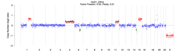
Multiple output files are produced, “seg.txt” contains the calls. Chromosome and genome-wide pdf images are also produced:

Methylation classification

Methylation data can be analysed using a range of third-party classification tools and workflow configurations. Central nervous system (CNS) tumour classification tools often rely on the data used in Capper et al, (Nature, 2018) which was based on EPIC array CpG sites. Classifiers that support Oxford Nanopore sequencing generally only use methylation calls at these sites as they use the original classifier model.

A range of different machine learning approaches are used for classification.

Considerations when selecting a classifier:

• Rapid classification during sequencing or post-run classification. Some classifiers work on one or the other; others work on both types.

• Adaptive Sampling or shallow genome. Some classifiers work on one or the other; others work on both types.

• CLI or GUI. Most tools are run directly from the command line (CLI). However, there are some graphical user interface (GUI) tools available.

The accuracy and confidence of tumour methylation classification is dependent upon many different factors including the tumour content of the sample, DNA quality, how well the training set covers that tumour type and the chosen classifier, etc. Some users choose to run one classifier; others adopt a consensus approach of using two or more.

Note that many of these tools have very strict licensing terms.

All tools listed here start from nanopore mod-bam files (base modifications are captured in the BAM file), but several have pre-processing steps before classification.

A neural network CNS-only classifier that works in Adaptive Sampling and shallow genome modes, and can be run as ultra-rapid live analysis and post-sequencing.

Link: Sturgeon

Type: CLI

Pre-processing: The Sturgeon documentation recommends using chm13v2.0_T2T-aligned BAM as input. We have used the GRCh38-aligned BAM with the hg38 parameter available without any issues. Process with Modkit following the Sturgeon online instructions of which we have examples below, then run the Sturgeon classifier.

Download code:

Branch: master Tag: 
v0.4.4
Date accessed: 2026-04-27

git clone https://github.com/marcpaga/sturgeon
cd sturgeon

Create environment:

python3.9 -m venv venv source   
venv/bin/activate
pip install . --no-cache-dir

Download model from here:

wget -O general.zip https://www.dropbox.com/s/yzca4exl40x9ukw/general.zip?dl=1

Prepare the data:

Change input.bam, output.txt and output.bam in commands below. Make sure input.bam is in its own folder so that all inputs and analyses are within the same sample folder.

wget https://github.com/nanoporetech/modkit/releases/download/v0.6.1/modkit_v0.6.1_u16_x86_64. tar.gz
tar -xvzf modkit_v0.6.1_u16_x86_64.tar.gz
./dist_modkit_v0.6.1_481e3c9/modkit adjust-mods --convert h m <input.bam> <output.bam>
./dist_modkit_v0.6.1_481e3c9/modkit extract full <output.bam> <output.txt>

sturgeon inputtobed -i <input_dir> -o <output_prefix> -s modkit --reference-genome hg38

Run the classifier:

sturgeon predict -i output_prefix -o <prefix_results/> --model-files ./general.zip --plot-results

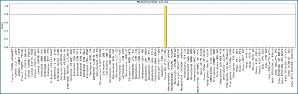
A csv file provides the prediction. The same information is plotted and provided in a pdf:

A pipeline that runs the crossNN neural network classifier for CNS tumours, along with ichorCNA to provide copy number calls and a genome-wide plot. It works with Adaptive Sampling and shallow whole-genome sequencing data, and is run post-sequencing.

Link: NanoDx

Type: CLI

Pre-processing: Supports hg19. Provide unaligned BAM.

Download code:

Branch: master Tag: 
v1.2
Date accessed: 2026-04-27

git clone https://gitlab.com/pesk/nanoDx.git cd nanoDx/

Requires hg19 reference use which needs to be unzipped and fai indexed:

wget https://hgdownload.cse.ucsc.edu/goldenpath/hg19/bigZips/hg19.fa.gz

gunzip hg19.fa.gz

Assuming you have samtools on command line or activate a conda env:

samtools faidx hg19.fa.

Download and move model to correct location:

wget -O files-archive.zip https://zenodo.org/api/records/14006255/files-archive mkdir models

mv files-archive.zip ./models/

unzip ./models/files-archive.zip

Conda install:

conda config --set channel_priority strict

conda create -n nanoDx -c conda-forge -c bioconda snakemake=7.32.4 python=3.11 conda activate 

nanoDx

May be required:

pip install pod5

If mapped, unalign the BAM for the pipeline to convert and remap:

samtools reset -@ 24 --no-PG --no-RG -o <output.bam> <input.bam>

Run classifier:

Note the < sample > needs to be the folder name of where your BAM is in relation to the folder you give in the config so results/ in config and < VQL > would be results/VQL/ is where the unaligned BAM is found with none_bam.

snakemake --use-conda --conda-frontend conda -
c 1 results/reports/<sample>_WGS_report_Capper_et_al.pdf

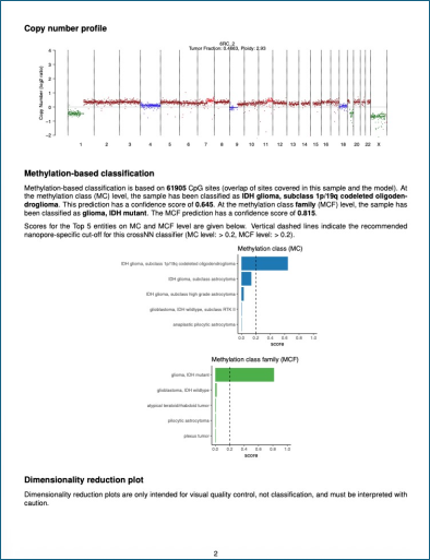
The classifications are provided in tsv and txt format, along with a more extensive pdf report:

Commercial software that implements both Sturgeon (the production-grade original methylation prediction model, also available on GitHub, see above), Marlin and Lamprey (specialized classifiers for leukaemia molecular diagnosis), and the Epinn models, which include Argus-CNS, Epinn-OSCC (an alpha model for oral squamous cell carcinoma), and works in Adaptive Sampling and shallow genome modes, run both rapidly and post-sequencing.

Link: Epinn

Type: GUI (local compute)

Pre-processing: None: point to bam_pass folder (GRCh38)

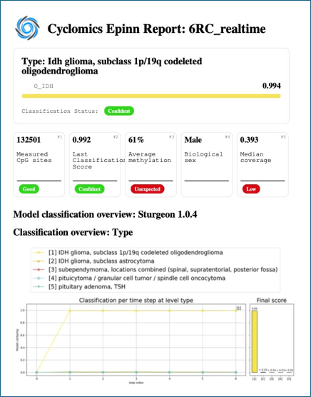
From the Epinn interface, you can opt to produce a pdf report:

Academic software that wraps multiple tools for rapid analysis into a GUI, containing CNS classifiers, Sturgeon and nanoDx and identifying copy number events and gene fusions. It can be used in Adaptive Sampling mode, to either analyse rapidly or post-run.

Link: ROBIN, User guide

Type: GUI (local compute)

Pre-processing: None: point to bam_pass folder

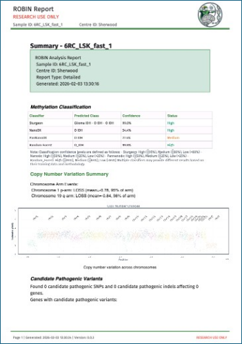
To note:

• ROBIN v0.5 supports BAM files containing up to 50,000 reads, including supplementary alignments. As MinKNOW excludes supplementary alignments from read counts, we recommend configuring MinKNOW to write 35,000 reads per file. Exceeding the supported read count may result in delayed classifications.

• We recommend running ROBIN using external (not sequencing instrument) compute.

• To run in rapid mode, data should be streamed off the device and into a location that is visible to ROBIN.

• Please refer to the Ultra-rapid singleplex Adaptive Sampling protocol for guidance on appropriate MinKNOW settings for this.

• Additionally, follow MinKNOW setup instructions for ROBIN to avoid sequencing issues.

These tools are also available but have not been evaluated.

RapidCNS2

Application

A wrapper based on nanoDx that runs several tools, including CNS classifier, and produces a report, and works in Adaptive Sampling mode with rapid analysis.

Tools

Link: RapidCNS2

Type: CLI

Required inputs

Pre-processing: Refer to the documentation.

Notes

A commercial licence is required for some components e.g. ANNOVAR has to be licensed from Qiagen.

Epignostix/MNP-Flex

Application

Epignostix/MNP-Flex is a commercial sarcoma or CNS tumour classifier developed using the Heidelberg CNS classifier model, that was trained on large reference cohorts.

Tools

Link: Epignostix/MNP-Flex

Type: GUI (web page upload)

Required inputs

Pre-processing: Refer to the documentation once logged into the website, contained within the Download resources section.
Process with Modkit following the tools’ online instructions, then upload a subset BED file.

Notes

Commercial software. A script is available from Epignostix to process bedMethyl file into the appropriate format for upload into the classifier. Important parameters to use with Modkit are --combine-mods.

Users are responsible for ensuring that the computational infrastructure, software configuration, and performance characteristics of any third-party bioinformatics tools are appropriate for their intended use.

Oxford Nanopore recommends consulting the relevant tool documentation and contacting the tool developers directly for further guidance on system requirements, installation, validation, and supported use cases.

Workflows

The wf-somatic-variation, a Nextflow workflow developed by Oxford Nanopore, can be used to call SNV and SV in both whole genome sequencing and Adaptive Sampling data. It runs ClairS/ClairS-TO and Severus.

wf-somatic-variation

Note: The workflow picks the ClairS-TO model from the basecaller model recorded in the input BAM/CRAM headers. If your data was basecalled with a model that ClairS-TO does not support, or a newer one that it does not recognise, use --override_basecaller_cfg to choose the closest appropriate model that ClairS-TO provides.

Example (ClairS-TO model for Dorado v4.2.0 SUP):

--override_basecaller_cfg 'dna_r10.4.1_e8.2_400bps_sup@v4.2.0'

The override only changes where ClairS-TO model is used. It does not need to match your actual basecalling model exactly. If your data was basecalled with a newer model than ClairS-TO supports, pick the newest model ClairS-TO provides rather than an older one.

There are a number of third-party workflows that can be used for variant calling and/or classification of tumour samples. Some are listed here but have not been evaluated in detail. Note that some may not be appropriate for use in Adaptive Sampling; they may be intended for deep whole genome sequencing only.

Variant calling	Methylation classification
DIANA DIANA is designed for WGS but uses the BED file for SNV calling and QNDAseq for CNV calling. Relevant publication	DIANA DIANA is designed for WGS but uses the BED file for SNV calling and QNDAseq for CNV calling. Relevant publication
nf-core-oncoseq	nf-core-oncoseq
NASVAR NASVAR is designed for tumour-only Adaptive Sampling and detects SNVs, CNVs, fusions, and ITDs.
Lrsomatic
Lumos

Workflow	SNV	SV	CNA	MGMT status	Classification
DIANA	x	x	x	x	x
nf-core-oncoseq	x (BED file required)	x (BED file required)	x		x
NASVAR	x (BED file required)	x (BED file required)	x
Epinn			x	x	x
ROBIN			x		x
Lrsomatic	x	x	Not suitable for AS
Lumos	x	x	Not suitable for AS
Epignostix				x	x
nanoDx			x		x
RapidCNS2	x	x	x	x	x
wf-somatic-variation	x	x

Data QC

This section captures some commands that may be useful for performing basic QC of an Adaptive Sampling experiment.

The reference alignment section of the HTML report from MinKNOW provides coverage across the entire reference genome and can therefore be used as an indicator of off-target coverage.

The BED regions section provides coverage for the regions specified in the BED file. For Adaptive Sampling analyses, these regions may appear twice, once for the forward strand and once for the reverse strand. This duplication reflects the strand-specific BED representation only; coverage is still calculated from reads aligned to both strands. Therefore, one of the duplicated rows is sufficient for interpretation.

As these reported regions include the Adaptive Sampling buffer region around the intended target, with coverage often decreasing toward the region boundaries, the displayed values may not reflect the coverage of the true biological target precisely. In many cases, the actual target region will have higher coverage than is suggested by the HTML report.

To calculate the true on-target coverage, run mosdepth using the gene target BED file:

mosdepth --by genes.bed sample_name aligned_reads.bam

The resulting output provides per region coverage metrics for the specified targets and is a more accurate measure of on-target performance.

For on-target coverage (per BED region), the main file needed from the mosdepth output is:

• sample_name.regions.bed.gz

This contains one row per region from your BED file with a coverage value. The key column is the mean coverage for each region.

Example columns:

chrom start end region_name mean_coverage

To calculate read length statistics for on-target reads, you can subset reads overlapping your target regions and summarise their lengths using samtools and seqkit.

samtools view -L genes.bed -b aligned_reads.bam | samtools fasta - | seqkit stats -a

This command:

• Extracts reads overlapping the regions defined in targets.bed
• Converts them to FASTA format
• Reports summary statistics including mean read length, N50, and minimum/maximum read lengths

The output provides a concise overview of read length characteristics for on-target reads and can be used to assess enrichment performance.

Enrichment can be estimated as the ratio of total bases sequenced on-target versus off-target:

enrichment = total on-target bases / total off-target bases

Note: You should use the buffered targets BED file and not the genes BED (targets only) file for the calculation as the buffer is part of the enrichment.

To perform the calculation, sum the read lengths for reads overlapping the target regions (on-target) and those that do not (off-target).

• Step 1: Calculate on-target bases

samtools view -L targets.bed aligned_reads.bam | \
awk '{on += length($10)} END {print "on-target bases:", on}'

• Step 2: Calculate off-target bases

samtools view -L targets.bed -b -U /dev/stdout aligned_reads.bam > /dev/null |\samtools view - | \
awk '{off += length($10)} END {print "off-target bases:", off}'

• Step 3: Calculate enrichment

On-target percentage = (on-target bases / (on-target bases + off-target bases)) x 100

Fold enrichment = (on-target bases / (on-target bases + off-target bases)) / (target size / genome size)

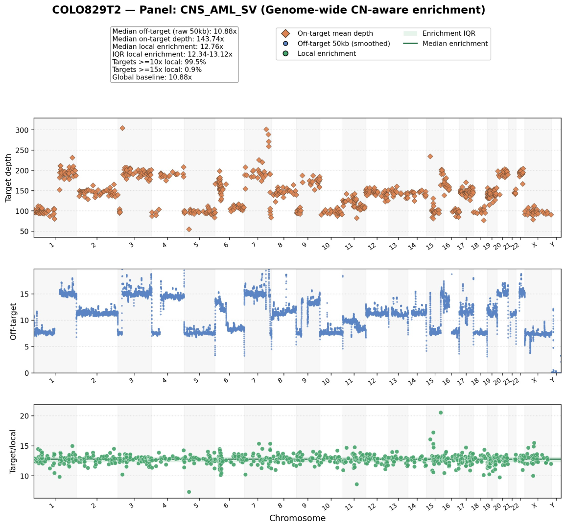
The plotting workflow expects two precomputed mosdepth region files from the same BAM:

• One target-level *.regions.bed.gz file generated by running:

mosdepth --by <targets BED>

• One fixed-width genome-wide *.regions.bed.gz file generated by running:

mosdepth --by <window size>

The resulting figure contains:

• An on-target depth panel
• An off-target depth panel
• An optional target/local enrichment panel

The workflow accepts any fixed-width genome-wide mosdepth window size. The window size does not need to be limited to 50 kb or 1 Mb, and it is not necessary to generate both for a given sample.

• 50 kb windows are a good choice when the local enrichment panel is important and a more local background estimate is desired.
• 1 Mb windows are useful for a coarser off-target overview.
• Other fixed-width values are supported. In practice, the choice should reflect the desired visual granularity and the level of local background structure that needs to be retained.

The script infers the actual off-target window size from the supplied mosdepth file and adjusts smoothing accordingly.

Environment creation

conda create -n as_covplot -c conda-forge -c bioconda python=3.12 numpy matplotlib mosdepth -y 
conda activate as_covplot

conda activate as_covplot

Inputs

BAM=/path/to/sample.aligned.bam TARGETS_BED=/path/to/adaptive_sampling_targets.bed
CEN_MASK=/path/to/grch38.cen_coord.curated.bed 
SAMPLE_ID=SAMPLE_ID PANEL_NAME=PANEL_NAME 
ROOT=/path/to/coverage_plot_run MOSDEPTH_DIR=${ROOT}/mosdepth 
PLOT_DIR=${ROOT}/plots 
LOG_DIR=${ROOT}/logs PLOT_SCRIPT=plot_target_enrichment_coverage_fixed.py

• TARGETS_BED should be the BED used to define the Adaptive Sampling targets (targets only, not buffer, no strand specificity).
• CEN_MASK is optional and is only needed when generating a centromere masked off-target panel.

Step 1: Generate mosdepth inputs

Generate one target-level mosdepth file and one fixed-width genome-wide mosdepth file from the same BAM.

mkdir -p "${MOSDEPTH_DIR}" "${PLOT_DIR}" "${LOG_DIR}"

TARGET_PREFIX="${MOSDEPTH_DIR}/${SAMPLE_ID}.targets"      WINDOW_PREFIX="${MOSDEPTH_DIR}/${SAMPLE_ID}.window_CHOSEN"
mosdepth -x -t 8 --no-per-base --by "${TARGETS_BED}" "${TARGET_PREFIX}" "${BAM}" mosdepth -x -t 8 --no-per-base --by CHOSEN_WINDOW_SIZE_BP "${WINDOW_PREFIX}" "${BAM}"                                                                     

This produces the required plotting inputs:

${TARGET_PREFIX}.regions.bed.gz 
${WINDOW_PREFIX}.regions.bed.gz

Step 2: Generate the plot

Run the plotting script using the target-level and fixed-width mosdepth outputs.

python "${PLOT_SCRIPT}" 

--target-regions "${TARGET_PREFIX}.regions.bed.gz" 

--window-regions "${WINDOW_PREFIX}.regions.bed.gz" 

--targets-bed "${TARGETS_BED}" 

--output-prefix "${PLOT_DIR}/${SAMPLE_ID}_coverage_plot" 

--sample-label "${SAMPLE_ID}" 

--panel-label "${PANEL_NAME}" 

--title-suffix "Genome-wide CN-aware enrichment" 

--format png 

--log-file "${LOG_DIR}/${SAMPLE_ID}_coverage_plot.log"

To hide centromeric bins from the off-target panel, add:

--offtarget-mask-bed "${CEN_MASK}"

Current plotting behaviour

Target-depth panel: full observed y-range by default

Off-target panel: percentile-derived y-range by default

Local-enrichment panel: full observed y-range by default

Current smoothing defaults use an approximate 1 Mb smoothing span, resolved against the supplied off-target window size.

50 kb windows resolve to 21 smoothing bins.

1 Mb windows resolve to 1 smoothing bin.

The optional centromere mask only affects the displayed off-target panel. It does not change the local background calculation used for the target/local enrichment panel.

Expected outputs

Expected figure output:

${PLOT_DIR}/${SAMPLE_ID}_coverage_plot.png

When --write-sidecars is used, the script also writes:

.per_target_coverage_with_local_background.csv
.offtarget_precomputed.csv
.summary.json

Example output:

Branch: master Tag: 
v0.4.4  
Date accessed: 2026-04-27 

git clone https://github.com/marcpaga/sturgeon cd sturgeon 

wget -O general.zip https://www.dropbox.com/s/yzca4exl40x9ukw/general.zip?dl=1 
venv/bin/activate
pip install . --no-cache-dir

sturgeon predict -i output_prefix -o <prefix_results/> --model-files ./general.zip --plot-results

tar -xvzf modkit_v0.6.1_u16_x86_64.tar.gz
./dist_modkit_v0.6.1_481e3c9/modkit adjust-mods --convert h m <input.bam> <output.bam> 
./dist_modkit_v0.6.1_481e3c9/modkit extract full <output.bam> <output.txt> 

sturgeon inputtobed -i <input_dir> -o <output_prefix> -s modkit --reference-genome hg38 

Branch: master Tag:   
v1.2                                       
Date accessed: 2026-04-27 

git clone https://gitlab.com/pesk/nanoDx.git 
cd nanoDx/ 

conda config --set channel_priority strict 

conda create -n nanoDx -c conda-forge -c bioconda snakemake=7.32.4 python=3.11 conda activate 

nanoDx

pip install pod5 

snakemake --use-conda --conda-frontend conda -
c 1 results/reports/<sample>_WGS_report_Capper_et_al.pdf 

Troubleshooting

Problem

Some BAM files contain header and read annotations that can cause readCounter or ichorCNA pre-processing to fail. This is usually caused by extra BAM header records or contigs that are not expected by the ichorCNA/readCounter workflow.

In particular, problems can occur when the BAM contains:

• @RG read group header lines
• @PG program header lines
• Non-primary contigs such as decoys, alternate haplotypes, unplaced contigs, or viral contigs
• Reads carrying RG:Z: tags
• Chromosome names outside the expected primary chromosome set

The fix is to create a cleaned BAM containing only the primary chromosomes and a simplified BAM header.

Create a clean BAM for ichorCNA/readCounter

Set the input and output paths:

BAM="input.bam"
CLEAN_BAM="input.clean.bam" 
HEADER_FILE="input.clean.header.bam"

Set the chromosome pattern to keep. For BAMs using chr chromosome names:

PRIMARY_CHROMS_REGEX='chr([1-9]|1[0-9]|2[0-2]|X|Y)'

For BAMs using non-chr chromosome names:

PRIMARY_CHROMS_REGEX='([1-9]|1[0-9]|2[0-2]|X|Y)'

Create a cleaned header by removing @RG and @PG lines and keeping only primary chromosome @SQ lines:

samtools view -H "${BAM}" \
| awk -v regex="${PRIMARY_CHROMS_REGEX}" 'BEGIN{OFS="\t"}
    /^@RG/ {next}
    /^@PG/ {next}
    /^@SQ/ {
        keep = 0
        for (i = 1; i <= NF; i++) {
            if ($i ~ "^SN:" regex "$") {keep = 1
            }
        }
        if (keep == 1) print next
    }
    {print}
' \
> "${HEADER_FILE}"

Check that the cleaned header was created:

if [[ ! -s "${HEADER_FILE}" ]]; then
   echo "ERROR: Clean header file was not created or is empty: ${HEADER_FILE}" >&2 exit 1
fi

Create the cleaned BAM by removing header lines from the alignment stream, keeping only reads mapped to primary chromosomes, removing RG:Z: tags, then adding the cleaned header back:

samtools view -h "${BAM}" \
| awk -v regex="${PRIMARY_CHROMS_REGEX}" 'BEGIN{OFS="\t"}
    /^@/ {next}
    $3 !~ regex {next}
    {
        out = ""
        for (i = 1; i <= NF; i++) {if ($i !~ 
             /^RG:Z:/) {
                out = (out == "" ? $i : out OFS $i)
            }
        }
        print out
    }
' \
| cat "${HEADER_FILE}" - \
| samtools view -b -o "${CLEAN_BAM}" -

Check and index the cleaned BAM:

if [[ ! -s "${CLEAN_BAM}" ]]; then
   echo "ERROR: Failed to create cleaned BAM: ${CLEAN_BAM}" >&2
   exit 1
fi

samtools index "${CLEAN_BAM}" || {
   echo "ERROR: Failed to index cleaned BAM: ${CLEAN_BAM}" >&2
   exit 1
}

The cleaned BAM can then be used as input to the ichorCNA/readCounter step:

readCounter \
  --window 1000000 \
  --quality 20 \
  --chromosome    "chr1,chr2,chr3,chr4,chr5,chr6,chr7,chr8,chr9,chr10,chr11,chr12,chr13,chr14,chr15,chr16,chr17,chr18,chr19,chr20,chr21,chr22,chrX,chrY" \
  "${CLEAN_BAM}" \
  > sample.wig

Important notes

This cleaning step does not realign the BAM and does not change read coordinates. It only removes unsupported header records, non-primary contigs, and read group tags that may interfere with ichorCNA/readCounter.

Use the chromosome regex that matches the BAM naming convention. For example, use the chr1 style regex for BAMs aligned to references with chr prefixes, and the 1 style regex for BAMs aligned to references without chr prefixes.

The cleaned BAM should only be used when the BAM and ichorCNA resources are based on the same genome build.

Problem

In some installations, running the original ichorCNA runIchorCNA.R file directly with Rscript may appear to do nothing, or may fail because expected helper functions are not available.

This can happen when the original runIchorCNA.R file mainly defines the ichorCNA workflow function, such as run_ichorCNA(), but does not actually call that function when executed from the command line. It may also assume that other ichorCNA helper scripts have already been sourced into the R session.

Symptoms can include:

• The script exits without producing expected output files.
• No ichorCNA plots, segments, or results are written.
• Helper functions such as getSeqInfo() are missing.
• The script behaves differently when sourced interactively compared with being run by Rscript.
• The original ichorCNA file loads successfully but the analysis itself is never started.

Why this happens?

The ichorCNA workflow is split across several R helper files. The main runIchorCNA.R script depends on functions from files such as:

• utils.R
• segmentation.R
• plotting.R
• plotIchorCNAzoom.R
• output.R
• EM.R
• createPanelOfNormals.R

Depending on how ichorCNA was installed or copied, these helper files may not be automatically loaded before runIchorCNA.R is used.

In addition, the original script may define the function run_ichorCNA() without executing it directly. In that situation, Rscript runIchorCNA.R ... can complete without actually running the analysis.

Solution

Use the patched wrapper script runIchorCNA.with_helpers.R instead of calling the original runIchorCNA.R directly.

The wrapper script makes the command line execution explicit. It:

1. Checks that the required R packages are installed.
2. Sources the ichorCNA helper files from the same directory as the script.
3. Checks that key helper functions have been loaded.
4. Sources the original runIchorCNA.R
5. Checks that run_ichorCNA() exists.
6. Parses the command line arguments.
7. Calls run_ichorCNA() directly.

This means the wrapper does not replace the ichorCNA algorithm. It simply ensures that the original ichorCNA code is loaded correctly and then actually launches the analysis.

Example command

Rscript ./ichorCNA/scripts/runIchorCNA.with_helpers.R \
 --id SAMPLE \
 --WIG  ./test60/ichorCNA_results/060min/wig/ \
 --gcWig ./ichorCNA/inst/extdata/gc_hg38_1000kb.wig \
 --mapWig ./ichorCNA/inst/extdata/map_hg38_1000kb.wig \
 --centromere ./ichorCNA/inst/extdata/GRCh38.GCA_000001405.2_centromere_acen.txt \
 --normal 0.40 \
 --estimateNormal FALSE \
 --ploidy "c(2,2.5,3)" \
 --sex male \
 --normalizeMaleX TRUE \
 --maxCN 6 \
 --chrs "c(1:22,'X')" \
 --chrTrain "c(1:22)" \
 --genomeBuild hg38 \
 --genomeStyle UCSC \
 --estimatePloidy TRUE \
 --estimateScPrevalence TRUE \
 --normalPanel None \
 --plotFileType pdf \
 --outDir ./test

Important notes

The wrapper script does not modify the WIG input, the reference files, or the ichorCNA model. It only fixes how the R code is loaded and executed.

The original runIchorCNA.R file is still used. The wrapper sources it and then calls run_ichorCNA() explicitly.

The wrapper should be kept in the same directory as the original ichorCNA helper scripts, otherwise it may not be able to find files such as utils.R, segmentation.R, or plotting.R.

If the wrapper reports missing R packages, install those packages into the active conda/R environment before rerunning.

If the wrapper reports that getSeqInfo() or run_ichorCNA() is missing, check that the script is in the correct ichorCNA scripts directory and that the original helper files are present.

This issue is separate from BAM/header problems during readCounter. The wrapper helps with running the ichorCNA R analysis after the WIG file has already been created.